IncliNET

1. Introduction
2. Data Preparation
   • 2.1. Inclination Labels
     • 2.1.1. Comparing users' adjusted measurements against each other
     • 2.1.2. Notebooks
   • 2.2. Image Extraction
   • 2.3. Image Augmentation
     • 2.3.1. Notebooks
3. Models
   • 3.1. Model 4
   • 3.2. Model 5
   • 3.3. Model 6
4. Training
   • 4.1. Regression, determining inclinations
     • 4.1.1. Notebooks
     • 4.1.2. Challenges
     • 4.1.3. Notes
     • 4.1.4. Pros
     • 4.1.5. Cons
     • 4.1.6. Plotting the evaluation metrics
   • 4.2. Classification, determining good/bad galaxy images
     • 4.2.1. Notebooks
     • 4.2.2. Plotting the evaluation metrics
5. Testing
   • 5.1. Comparing the Regression Models
   • 5.2. Visualizing the outliers
   • 5.3. Averaging models
   • 5.4. The power of bagging
   • 5.5. Evaluation of the Binary Models
   • 5.6. Summary
6. Deliverable Products
   • 6.1. Model Production Pipeline
     • 6.1.1. Orchestration
     • 6.1.2. Retraining Strategy
     • 6.1.3. Suggestions to Improve Models
   • 6.2. Deployment
     • 6.2.1. Code Repository & Issues
     • 6.2.2. Installation
   • 6.3. Web Application
   • 6.4. API
7. Documentation
8. Acknowledgments
   • 8.1. About the data
   • 8.2. Citation
   • 8.3. Author
   • 8.4. Disclaimer
9. References

1. Introduction

The inclination of spiral galaxies plays an important role in their astronomical analyses such as measuring their distances using the correlation between their rotation rates and absolute luminosities. Each galaxy has its own unique morphology, luminosity, and surface brightness profiles. In addition, galaxy images are covered by foreground stars of the Milky Way galaxy. Therefore, it is challenging to design an algorithm that automatically determines the 3D inclination of spiral galaxies. The inclinations of spiral galaxies can be coarsely derived from the ellipticity of apertures used for photometry, assuming that the image of a spiral galaxy is the projection of a disk with the shape of an oblate spheroid. For ~1/3 of spirals, the approximation of axial ratios provides inclination estimates good to better than 5 degrees, with degradation to ~5 degrees for another 1/3. However in ~1/3 of cases, ellipticity-derived inclinations are problematic for a variety of reasons. Prominent bulges can dominate the axial ratio measurement. Some galaxies may not be axially symmetric due to tidal effects. High surface brightness bars within much lower surface brightness disks can lead to large errors. Simply the orientation of strong spiral features with respect to the tilt axis can be confusing. The statistical derivation of inclinations for large samples has been unsatisfactory.

The task of manual evaluation of galaxy inclinations is tedious and time consuming. In the future, with the large astronomical survey telescopes coming online, this task could not be efficiently done manually for thousands of galaxies. The objective of this project is to automatically determine the inclination of spiral galaxies with the human level accuracy providing their images, ideally in both colorful and black-and-white formats.

Our collection of carefully measured inclinations provides a rich data set for training a machine-learning algorithm, such as the Convolutional Neural Network (CNN), to replace the human eye in future projects. To successfully instruct such a network to produce satisfactory results, a training set of order ~10,000 representative galaxies is required. Our entire sample is of such a size, and hence suitable for exploring machine-learning capabilities. Moreover, n-body cosmological simulations such as Illustris provide exquisite images of projected spiral galaxies with known 3D orientations that could be of potential interest as training sets for inclination studies.

2. Data Preparation

2.1. Inclination Labels

We have investigated the capability of the human eye to evaluate galaxy inclinations. We begin with the advantage that a substantial fraction of spiral inclinations are well defined by axial ratios. These good cases give us a grid of standards of wide morphological types over the inclination range that particularly interests us of 45-90 degrees. The challenge is to fit random target galaxies into the grid, thus providing estimates of their inclinations.

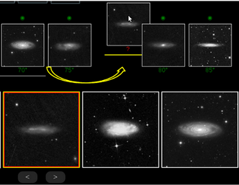
Fig. 1: Users compare each target galaxy with a set of standard galaxies to evaluate their inclinations.

To obtain a large enough sample for an ML project, we have manually labelled ~20,000 spiral galaxies using an online GUI, Galaxy Inclination Zoo, in collaboration with amateur astronomers across the world. In this graphical interface, we use the colorful images provided by SDSS as well as the g, r, i band images generated for our photometry program. These latter are presented in black-and-white after re-scaling by the asinh function to differentiate more clearly the internal structures of galaxies. The inclination of standard galaxies were initially measured based on their axial ratios. Each galaxy is compared with the standard galaxies in two steps (see Fig. 1). First, the user locates the galaxy among nine standard galaxies sorted by their inclinations ranging between 45 degrees and 90 degrees in increments of 5 degrees. In step two, the same galaxy is compared with nine other standard galaxies whose inclinations are one degree apart and cover the 5 degree interval found in the first step. At the end, the inclination is calculated by averaging the inclinations of the standard galaxies on the left/right-side of the target galaxy. In the first step, if a galaxy is classified to be more face-on than 45, it is flagged and step two is skipped. We take the following precautions to minimize user dependent and independent biases:

• We round the resulting inclinations to the next highest or smallest integer values chosen randomly.
• At each step, standard galaxies are randomly drawn with an option for users to change them randomly to verify their work or to compare galaxies with similar structures.
• To increase the accuracy of the results, we catalog the median of at least three different measurements performed by different users.
• Users may reject galaxies for various reasons and leave comments with the aim of avoiding dubious cases.

The uncertainties on the measured inclinations are estimated based on the statistical scatter in the reported values by different users. Fig. 2 illustrates the distribution of labels, where J and F label rejected and face-on galaxies, respectively. Numbers indicate the inclination angle of galaxies from face-on in degrees. As seen, out of 19,907 galaxies, ~22% are rejected for various astronomical reasons and ~8% are face-on thus not acceptable for our original research purpose.

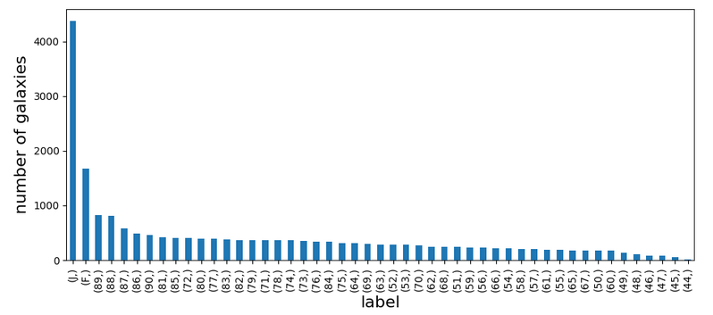
Fig. 2: The distribution of the labels across the sample

2.1.1. Comparing users' adjusted measurements against each other

This comparison is very similar to the A/B testing. Here, the only difference is that we divide users into two different groups, A and B. Then, we calculate the median of evaluated labels by these groups and compare the inclination of the common galaxies of both tables. This way, we are able to evaluate the statistical uncertainties on the measurements.

Fig. 3 compares the results of two different groups of users. Evidently, on average, the agreement between two different people about their inclination measurements y is ~3 degrees. Any machine learning tool that has almost the similar performance is acceptable for our purpose.

As expected, we see smaller scatter at larger inclination values towards the edge-on galaxies. Practically, it is much easier for users to recognize and evaluate edge-on galaxies, which fortunately is in the favor of our astronomy research. This explains why our sample mainly consists of edge-on galaxies. On the other hand, more scatter about less inclined galaxies (that indicate larger uncertainty on the measured values) and having much smaller number of evaluated galaxies in that region makes it hard for machine learning algorithms to learn from data and have accurate predictions when galaxies tend to be more face-on (smaller inclination values).

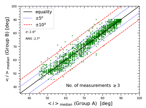
Fig. 3: Median of the evaluated inclinations by two different groups of users for ∼2000 galaxies.

2.1.2. Notebooks

For more details on how we have processed the ground truth results in order to avoid any human related mistakes or biases please refer to this notebook: https://github.com/ekourkchi/inclinet_project/blob/main/data_extraction/incNET_dataClean.ipynb

2.2. Image Extraction

To obtain the cutout image of each galaxy at g, r, and i bands, we download all corresponding calibrated single exposures from the SDSS DR12 database. We use MONTAGE, a toolkit for assembling astronomical images, to drizzle all frames and construct galaxy images. The angular scale of the output images is 0.4''/pixel. Our data acquisition pipeline is available online. For the task of manual labeling we presented images to users in 512x512 resolution. For the task of generating and testing multiple ML models, we degrade the resolution of images to 128x128. This allows us to make the project feasible given the available resources.

2.3. Image Augmentation

To avoid over-fitting, we increase the sample size by leveraging the augmentation methods. The inclination of each galaxy is independent of its projected position angle on the image and the image quality. Therefore, we augment our image sample by running them through a combination of transformations such as rotation, translation, mirroring, additive Gaussian noise, altering contrast, blurring, etc.

All image transformations that are applied in the augmentation process keep the aspect ratio of images intact to ensure that the elliptical shape of galaxies and their inclinations are preserved. The augmented sample is required to satisfy the following criteria

• The numbers of colorful (RGB) and grayscale (g, r, i) images are equal
• The numbers of black-on-white and white-on-black images are the same
• The g, r, and i-band images have equal chance of appearance in each batch

Fig. 4: Left: Distribution of the inclinations of the original sample galaxies. Right: Distribution of the augmented sample inclinations

Fig. 5 : Examples of augmented images. In each panel, galaxy ID is in cyan. Red is the inclination and magenta is the image pass-band, i.e. g, r, i and c, where c stands for RGB.

2.3.1. Notebooks

1. Here, data is processed for models to determine the inclinations of spiral galaxies by leveraging the regression methodologies. Fig.4 illustrates the distribution of inclinations in both original and augmented samples. Fig. 5 displays a subset of augmented images. https://github.com/ekourkchi/inclinet_project/blob/main/VGG_models/incNET_model_augmentation.ipynb

2. Here, data is processed for models that determine the usefulness of spiral galaxies for the task of evaluating inclinations by taking the classification approaches. Labels are presented in the binary form, where 0 denotes the accepted galaxies, and 1 represents the rejected ones due to various reasons, such as anomalies, ambiguities, or having poor quality or an unsatisfactory Hydrogen 21cm spectrum. A number of face-one galaxies (those with inclination lower than 45 degrees from face-on) that had originally passed our original sample selection criteria were also rejected. Fig. 6 illustrates the distribution of labels in the original and augmented samples. Fig. 7 shows a subset of augmented galaxies with their labels.
   https://github.com/ekourkchi/inclinet_project/blob/main/VGG_models/incNET_model_augmentation-binary.ipynb

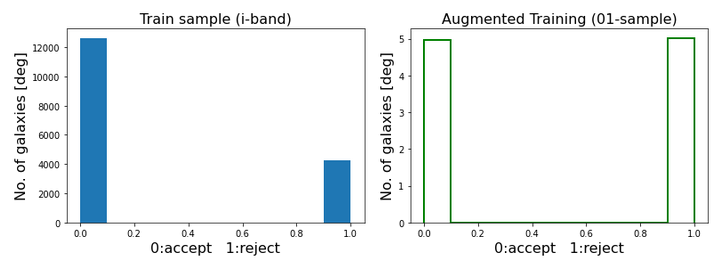
Fig. 6: Left: Distribution of the labels of the original sample galaxies. Right: Distribution of the sample labels after augmentation. Each batch covers both labels uniformly. This reduces any biases that originate from the data imbalance.

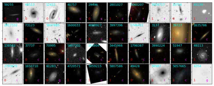
Fig. 7: Examples of augmented images. In each panel, the PGC ID of the galaxy is in cyan. Red is the classification label and magenta is the image pass-band, i.e. g, r, i and c, with c representing RGB images.

3. Models

Models have been define in this auxiliary code: https://github.com/ekourkchi/inclinet_project/blob/main/VGG_models/TFmodels.py

Our main objective is to evaluate the inclination of a spiral galaxy from its images, whether it is presented in grayscale or colorful. Moreover, we need to know what is the possibility of the rejection of a given image by a human user. Images are rejected in cases they have poor quality or contain bright objects that influence the evaluation process. Very face-on galaxies are also rejected.

We tackle the problem from two different angles.

1. To determine the inclination of galaxies, we investigate 3 models, each of which is constructed based on the VGG network, where convolutional filters of size 3x3 are used. The last layer benefits from the tanh activation function to generate numbers in a finite range, because the spatial inclination of our spirals falls into a finite range (45 to 90 degrees).

2. To determine the accept/reject labels, we build three other networks which are very similar to the regression networks except for the very last layer with the softmax activation function for binary classification.

Models have different complexity levels and are labeled as model4, model5 and model6, with model4 being the simplest one. In the following sections, we briefly introduce different models that we considered in this study.

For clarity, we label our models as model<n>(m), where<n> is the model label which can be 4, 5, and 6. <m> denotes the “flavor of the model”, where m=0 stands for a model that is trained utilizing the entire training sample. " represent models that have been trained using 67% of the data.

3.1. Model 4

This is the simplest model in our series of models. The total number of free parameters of this model is ~1.600,000. It consists of two sets of double convolutional layers. Fig. 8 visualizes the convolutional neural network of Mode 4.

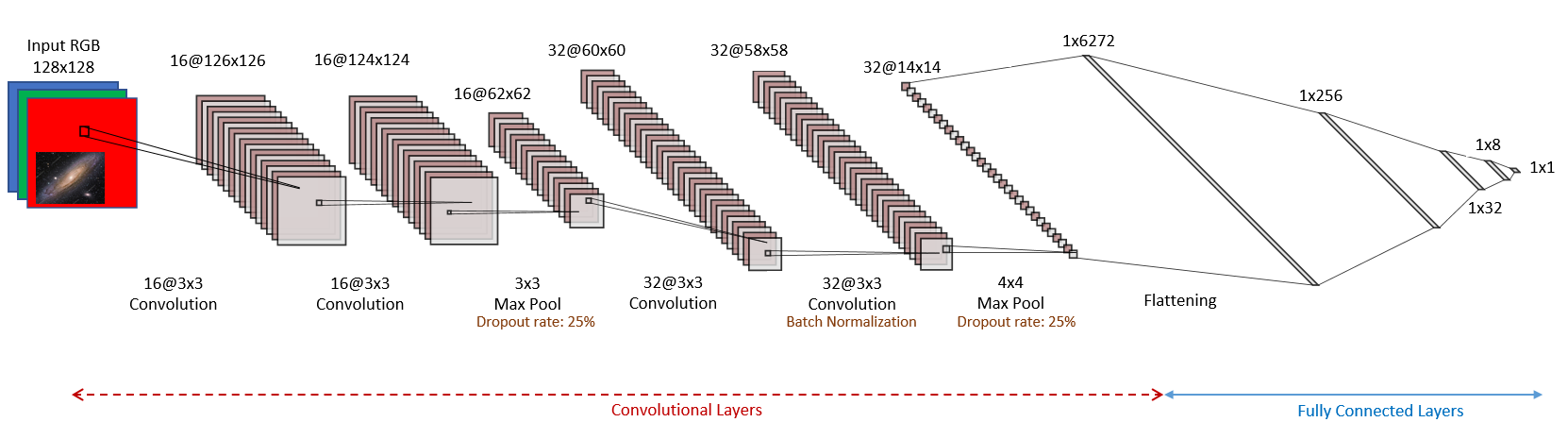
Fig. 8: The convolutional neural network of Model 4.

3.2. Model 5

This model is the most complex model in our study. It has ~2,500,000 free parameters and three sets of double convolutional layers.

3.3. Model 6

This model is comparable to Model4, in terms of complexity, although the number of convolutional units is larger in this model.

4. Training

Here, we train a VGG model using the augmented data. The data augmentation process has been explained above. The output augmented data has been stored on disk for the purpose of the following analysis. We set aside 10% of the sample galaxies for the purpose of testing (model evaluations).

4.1. Regression, determining inclinations

128x128 images are used for this analysis, which are in grayscale (g,r,i filter) or colorful (RGB). All images are presented in 3 channels. For grayscale images, all three channels are the same. Inclinations range from 45 to 90 degrees. Half of the grayscale images have black background, i.e. galaxies and stars are in white color while the background is dark. In half of the grayscale cases, objects are in black on white background. Half of the sample is in grayscale, and the other half is in grayscale. The augmentation process has been forced to generate images that cover the entire range of inclinations uniformly. We adopt the Adam optimizer, and the Mean Square Error (MSE) for the loss function, and we keep track of the MSE and MAE (Mean Absolute Error) metrics during the training process.

4.1.1. Notebooks

• Model 4: https://github.com/ekourkchi/inclinet_project/blob/main/VGG_models/128x128_Trainer_04.ipynb
• Model 5: https://github.com/ekourkchi/inclinet_project/blob/main/VGG_models/128x128_Trainer_05.ipynb
• Model 6: https://github.com/ekourkchi/inclinet_project/blob/main/VGG_models/128x128_Trainer_06.ipynb

4.1.2. Challenges

With 128x128 images, and adding augmentation, the size of the required memory to open up the entire augmented sample is out of the capability of the available machines (64 GB of RAM). Hence, we attempted to resolve the issue by storing the training sample in 50 separate batches on disk. All batches are already randomized in any way. Each step of the training process starts with loading the corresponding batch, reconstructing the CNN as it was generated in the previous iteration, and advancing the training process for one more step. At the end of that repetition, we store a snapshot of the network weights for the next training step.

4.1.3. Notes

• Since we are dealing with a large training sample, we need to repeat updating the network parameters for many steps to cover all training batches multiple times
• Over-fitting sometimes helps to minimize the prediction-measurement bias (this would be further discussed in the Testing section)

4.1.4. Pros

• We can generate as many training galaxies as required without being worried about the memory size
• We can stop the training process at any point and continue the process from where it is left. This helps if the process crashes due to the lack of enough memory that happens if other irrelevant processes clutter the system
• We are able to constantly monitor the training process and make decisions as it advances

4.1.5. Cons

• This process is slow. The bottleneck is the i/o processes, not training and updating the network parameters.

4.1.6. Plotting the evaluation metrics

As illustrated in Fig. 9, the training process can be stopped about the iteration #1000, however a little bit of over training helps to remove the prediction-measurement bias and reduces the magnitude of fluctuations in the evaluation metrics.

Fig. 9: Regression evaluations metrics vs. training epochs

4.2. Classification, determining good/bad galaxy images

To distinguish between accepted and rejected spiral galaxies for the purpose of our study, we train a VGG model using the augmented images that have been generated following the same procedure we explained in the previous section.

• 0: galaxy images with well-defined and measured inclinations, that are used for the distance analysis in a separate research
• 1: galaxies that are flagged to be either face-on (inclinations less than 45 degrees from face-on), or to have poor image quality. Deformed galaxies, non-spiral galaxies, confused images, multiple galaxies in a field, galaxy images that are contaminated with bright foreground stars have been also flagged and have label 1.

Here, we leverage the same networks we adopted for the inclination evaluation. For binary classification, the activation function of the last layer is replaced by the softmax function, and the network is trained with the sparse categorical entropy as the loss function. We keep track of the accuracy metric during the training process.

Objective: The goal is to train a network for automatic rejection of the unaccepted galaxies. These galaxies can be later manually studied or investigated by human users.

4.2.1. Notebooks

• Model 4: https://github.com/ekourkchi/inclinet_project/blob/main/VGG_models/128x128_Trainer_04-binary.ipynb
• Model 5: https://github.com/ekourkchi/inclinet_project/blob/main/VGG_models/128x128_Trainer_05-binary.ipynb
• Model 6: https://github.com/ekourkchi/inclinet_project/blob/main/VGG_models/128x128_Trainer_06-binary.ipynb

4.2.2. Plotting the evaluation metrics

According to Fig. 10, after about 200 iterations, the loss function of the training sample decreases while the performance gets worse on the validation sample. This means that over-training the network after this point doesn't improve the overall efficiency.

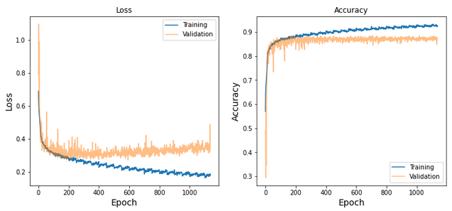
Fig. 10: classification evaluations metrics vs. training epochs

5. Testing

10% of the galaxies in our sample have been chosen and left out of the analysis for evaluating the performance of the models. The testing images are augmented in the same fashion by following the same recipe we used to prepare the training batches.

5.1. Comparing the Regression Models

Predictions vs. Actual measurements

We evaluate the performance of models based on the accuracy of their predictions. To better understand the performance of a model, we plot the differences between the evaluated inclinations and the manually measured values, i.e. ". In Fig. 11, the horizontal axis shows the measured inclinations. Each point represents a galaxy in the test sample.

• Left Panel: Predicted values , are directly generated by processing the testing sample through the same network. Red solid line displays the results of a least square linear fit on the blue points. Some models exhibit an inclination dependent bias that is inclination dependent. This bias has been linearly modeled by the red line, which is utilized to adjust the predicted values. The slope and intercept of the fitted line are encoded in the m and b parameters.

• Right Panel: Same as the left panel, but with the adjusted values, ", that is calculated using .

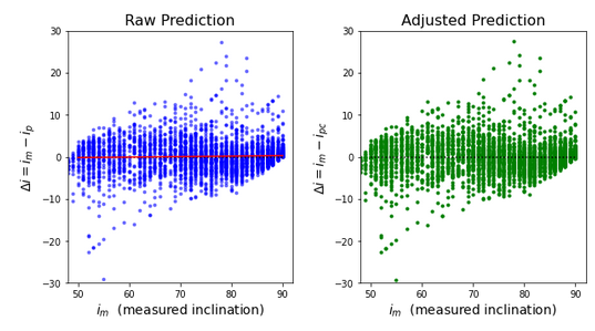
Fig. 11: Discrepancy between predictions and actual values for mode 4 with the test sample

The root mean square of the prediction-measurements differences is . The similar metric is when we compare the measured values of two groups of the human users. This means our model performs slightly worse than human, and most of that poor performance is attributed to the outliers and ano,aly features such as data noise, point sources, stellar spikes, poor images, etc. with not enough instances in the data sample to have significant influence on the trained network.

In a similar way, Fig. 12 compares the performances of all models. As seen, in almost all cases the prediction bias (the slope of the red line) is at minimum and not that significant. Each panel displays the results of one model, and is labeled with the name of the corresponding model. RMS and MAE denote “Root Mean Square” and “Mean Absolute Error” of the deviations of about zero. At first glance, Model5 seems to have the best performance, which does not come as a surprise, because it is the most complicated model, in terms of the number of free parameters. In general, the differences in the performances are not that significant.

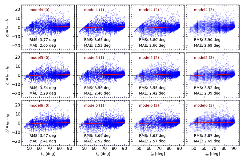
Fig. 12: The performance of all studied models using the test sample. Each panel illustrates the results of a model labeled as model<n>(m), with <n> being the model number which can be 4, 5, and 6. <m> denotes the “flavor of the model”, where m=0 stands for a model that is trained utilizing the entire training sample. represent models that have been trained using 67% of the data.

5.2. Visualizing the outliers

Fig. 13 displays the first 49 galaxy images in the test sample, where the predicted value is far from the actual measurements, i.e. "). In each panel, cyan label is the galaxy ID in the Principal Galaxy Catalog (PGC), and green and red labels represent the measured and the predicted inclinations. Magenta labels denote the panel numbers.

We attempt to check out the outliers and see if there is any noticeable similar feature or issues that might explain the poor outcome of the network. We look for noise levels, significant spikes, very bright stars or anything that might have distracted the network from producing the correct answer. Some cases are interesting:

• In panel #42, the galaxy image has been masked out because the bright center of the galaxy has saturated the image center.
• Case #26 is a typical case, where the galaxy image has been projected next to a bright star.
• Cases like #2, #14, #23, #29, #43 have poor quality images.
• Case #37 has been ruined in the data reduction pipeline, where the telescope images are preprocessed.

Fig. 13: Example of outliers for Model 4

5.3. Averaging models

We take two average types to combine the results of various models and possibly obtain better results, namely mean and median. We generate 4 sets of averages

• averaging the results of all model4 flavors (0, 1, 2, 3)
• averaging the results of all model5 flavors (0, 1, 2, 3)
• averaging the results of all model6 flavors (0, 1, 2, 3)
• averaging the results of all models with various flavors

We don't see any significant differences between mean and median, so there is no way we prefer one of them over the others. However, we recommend using the median just to ignore very severe outliers.

5.4. The power of bagging

As inferred from Figures 14 and 15, when the results of all models are averaged out, we get the best performance. The average of all models turns out to have the smallest deviations in the predicted-measured differences with the RMS and MAE of 3.09 and 2.12 [deg], respectively. This is relatively comparable with human performance.

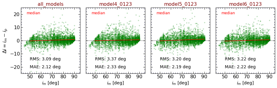
Fig. 14: Median of all predictions

Fig. 15: Mean of all predictions

5.5. Evaluation of the Binary Models

Three different metrics have been considered to evaluate the classification models, namely “precision”, “recall” and “accuracy”. These metrics are defined as

• precision = TP/(TP+FP)
• recall = TP/(TP+FN)
• accuracy = (TP+TN)/(TP+FP+FN+TN)

where TP and FP are true and false positives, respectively. In a similar way, TN and FN are true and false negatives, respectively. Precision measures how many of the positive predictions are actually positive. Recall indicates how many of the actual positive cases have been detected correctly. Accuracy shows the fractions of correct predictions in the entire sample. Fig. 16 visualizes these metrics for different classification models that we considered in this project.

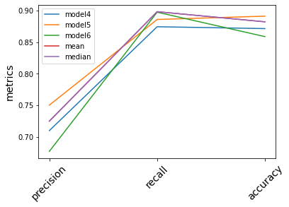
Fig. 16: The performance metrics of the various classification models in this study

Evidently, model5 has a better overall performance compared to the other two models, which is expected knowing that model #5 is the most complicated one. Averaging out the evaluated labels does make significant improvements, however model5 seems to perform slightly better than the average.

5.6. Summary

In this project, we trained three different convolutional neural networks (CNN) to automatically evaluate the inclination of the spiral galaxies. The performance of both classification and regression approaches have been extensively explored in the prototyping stage, where we conclude that all of the CNN models that end with a regression layer exhibit better performances.

Our exploratory data analysis reveals that the distribution of labels (inclinations) is not uniform. Although leveraging the tanh function for the activation of the last layer results in building good models, an inclination dependent bias is evident when we plot the discrepancies between the measured and predicted inclinations. We attributed this to the non-uniform distribution of inclinations and the fact that inclinations span a finite range of numbers between 45 and 90 degrees.

We modified our models by changing the activation of the last layer to Tanh. We normalized images and linearly adjusted inclination to be compatible with the Tanh output that ranges from -1 to 1. Although the bias is still evident, the convergence is achieved more quickly. Further tests seem to be necessary to make a concrete conclusion here.

We repeated the training process of the same CNNs (with Tanh output layer) by utilizing the augmented training samples that have uniform distributions of labels. We report a boost in the performances of our networks, while the prediction-measurement bias seems to be off less significance.

Using smaller batch sizes and training models with more iterations helped to minimize the bias. However, part of the bias that originates from the finite coverage of the inclinations could not be entirely removed.

Ultimately, this analysis recommends us to invoke the regression methodology to get more precise results. To minimize the bias, the labels of the training sample must be relatively uniform and Tanh helps with having better convergence rates through generating outputs in a finite range.

Footnote: Here, we prototyped three different models, all of which treat the problem as a regression problem: https://github.com/ekourkchi/incNET-data/blob/master/incNET_CNN_Colabs/Prototype_RGB64x64_VGGregression.ipynb . For the corresponding classification prototypes please refer to https://github.com/ekourkchi/incNET-data/blob/master/incNET_CNN_Colabs/Prototype_RGB64x64_VGGclassification.ipynb

6. Deliverable Products

The entire ML process is illustrated in Fig. 17. Left red block is the model production pipeline where the data is extracted, cleaned and prepared for training. The training process happens here. Right blue block illustrates the deployment unit, where the pretrained models are shipped to the deployment server that makes them available to users through a Web GUI and a REST API.

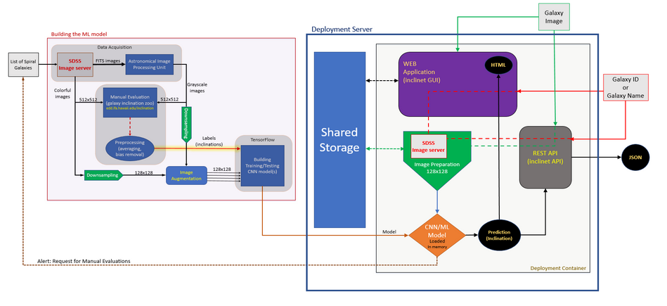
Fig.17: The ML process plan.

1. The Model Production Unit: This module consists of 4 main components:

• Data acquisition: Images are downloaded from the SDSS images web server (for this project we chose images taken from a specific telescope. For other telescopes, data acquisition and preprocessing might be different)
• Label generation: Galaxy images are evaluated by human users using an online GUI
• Image resizing and data augmentation: images are downsampled to the resolution of 128x128 to facilitate the training process, images are augmented to avoid overfitting
• ML model training/testing: CNN model(s) are trained and tested. Model(s) are then stored on disk and shipped to the deployment unit. Multiple models might be generated to compare their results at the deployment stage. If the results are far from each other, there would be an alarm going off asking for manual investigations to resolve the discrepancies.

2. Deployment Unit: The deployment has a monolithic architecture. The deployment container is executed on the deployment server and has access to the shared storage of the server through mounting the required folders.

• Shared Storage, stores the image products and log files of the online operation. Different components of the deployment container need the proper access to the storage to read and write data
• Deployment Unit: This is the heart of the service. The main component is developed using the Python package Flask. This unit hosts
  • Online web service, which includes a web application. Online users can communicate with the service through the online dashboard
  • API service, where users can send requests and images through a REST API
  • Models are preloaded into the deployment container. The CNN models reside in the memory as soon as the application is deployed, and there is no need to load them over at each API call. This accelerates the response time of the provided services
  • There is an image processing unit that prepares images to comply with the input format of the model network

6.1. Model Production Pipeline

The model production units and the corresponding ML pipeline are illustrated in Figures 18 and 19.

Visit this folder on gitHub for the codes: https://github.com/ekourkchi/inclinet_project/tree/main/production_pipeline

Fig. 18: The Model Production Unit

Fig. 19: ML pipeline

6.1.1. Orchestration

• Input Data
  • Data is presented in the form of images. Non-square images are padded to have square dimensions, and they are resized to the appropriate shape (128x128)
  • Labels are the spatial inclinations of spiral galaxies from face-on
• pipeline.sh: This bash script runs the pipeline end-to-end from the data preparation to building the CNN models
  • data_prep.py: This code is mainly used to downsize (downsample) images that are stored in a specified folder.
  • data_compress.py: compressing images of a folder that are all in the same size
  • data_split.py: taking the npz file at each filter, and splitting them into training and testing batches. 10% of all galaxies with inclinations greater than 45 degrees are set aside for the testing purpose. To perform extra analysis (like bagging), sub-samples of the training set are generated, with the size of 67% of the entire training sample size. Sub-samples overlap as each contains 2/3 of the data drawn randomly from the main sample, whereas the test sample doesn't overlap with any of the training sub-samples.
  • data_augment_uniform.py: Generating augmented samples with uniform distribution of inclination. The augmented samples are stored as batches for a later use in the training process. The training batches are generated using this code. Each batch consists of the same number of grayscale and colorful images. Half of the grayscale images are inverted to avoid overfitting
  • batch_training_regr.py: Training VGG models using the augmented data. Advancing the training process at each step consists of reconstruction of the model as it is at the end of the previous step. The steps of the training process are as follows
    • Reading the compressed files that holds the corresponding batch
    • Training the model for one epoch (moving forward just for 1 iteration)
    • Updating a JSON file that holds the network metrics at the end of the training epoch
    • Saving the weight values of the model for the use in the next iteration

6.1.2. Retraining Strategy

• This model has been trained using the SDSS data and therefore it performs very well on the similar data set. If data is generated using other telescopes or have very different color schema, then the model training needs to be revisited. Note that SDSS has not covered the entire sky, and mainly surveyed the northern sky (due to the geographic limitations of the telescope)
• In case of planning for the evaluation of a huge batch of new galaxies with very different types of data, the model needs to be tested in advance. If the performance is not satisfactory, for a small subset of images (~1,000 galaxies) the manual evaluation needs to be performed and retrain the model to adapt the new data.
• The retrained model would be shipped to the deployment container in h5 or pickled format.
• In the case of retraining, new data should be preprocessed to be compatible with our training pipeline. Each telescope and instrument has its own characteristics. The best practice is to generate 512x512 postage stamp images of galaxies through the telescope's APIs, or the FTP/HTTP services.

6.1.3. Suggestions to improve models

• One of the recommended methods is to create many synthetic galaxy images, with known inclinations. The results of galaxy simulations (such as Illustris) can be visualized at various spatial inclinations under controlled situations. Later, the resolution can be tuned to different levels and the foreground, background objects can be superimposed on the image. Additional noise and ambiguities can be added to images. All of these factors allow the network to gain enough expertise on different examples of galaxy images.
• To build more complicated models, we can present all images taken at different wavebands in separate channels, instead of parsing them as single entities. All passbands can be fed into the CNN at once.
• Images can be used in raw format. The dynamical range of the astronomical images are way beyond the 0-255 range. Instead of downscaling the dynamical range to produce visualizable images, one can use the full dynamical range of the observed images.

6.2. Deployment

Fig. 20 illustrates the deployment unit.

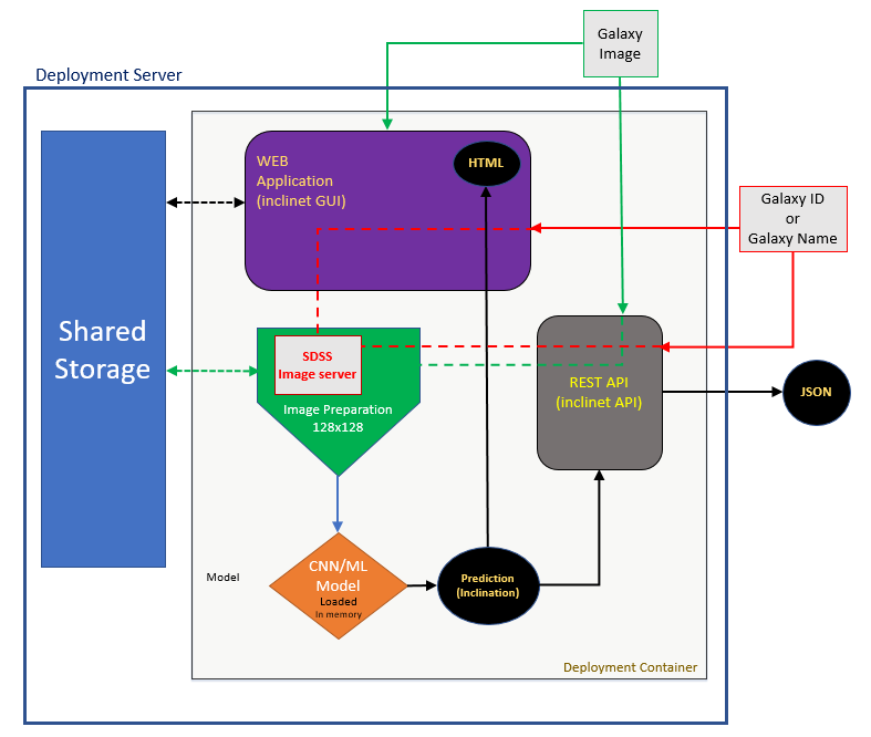
Fig. 20: The Deployment Unit. Galaxies are provided in forms of images or their ID in the PGC catalog

6.2.1. Code Repository & Issues

All deployment source codes are available on gitHub: https://github.com/ekourkchi/inclinet_deployment_repo

6.2.2. Installation

On a local machine using Docker

• First, you need to install Docker Compose.

pip install docker-compose

• Execute

$ docker run -it --entrypoint /inclinet/serverup.sh -p 3030:3030  ekourkchi/inclinet

• Open the Application: Once the service is running in the terminal, open a browser like Firefox or Google Chrome and enter the following url: http://0.0.0.0:3030/

On a server using Docker

• First, you need to install Docker Compose. How to install

• Execute

$ docker run -it --entrypoint /inclinet/serverup.sh --env="WEBROOT=/inclinet/" -p pppp:3030 -v /pathTO/public_html/static/:/inclinet/static ekourkchi/inclinet

where WEBROOT is an environmental variable that points to the root of the application in the URL path. pppp is the port number that the service would be available to the world. 3030 is the port number of the docker container that our application uses by default. /pathTO/public_html/static/ is the path to the public_html or any folder that the backend server uses to communicate with the Internet. We basically need to mount /pathTO/public_html/static/ to the folder inclinet/static within the container which is used internally by the application.

URL: Following the above example, if the server host is accessible through www.example.com, then our application would be launched on www.example.com/inclinet:pppp. Remember http or https by default use ports 80 and 443, respectively.

Directly from source codes

Just put the repository on the server or on a local machine and make sure that folder <repository>/static is linked to a folder that is exposed by the server to the outside world. Set WEBROOT prior to launching the application to point the application to the correct URL path.

Execution of server.py launches the application.

       $ python server.py -h
 
 
       - starting up the service on the desired host:port
      
       - How to run:
      
           $ python server.py -t <host IP> -p <port_number> -d <debugging_mode>
 
       - To get help
           $ python server.py -h
      
 
 
       Options:
       -h, --help            show this help message and exit
       -p PORT, --port=PORT  the port number to run the service on
       -t HOST, --host=HOST  service host
       -d, --debug           debugging mode
 

Please consult the IncliNET code documentation for further details. For more thorough details, refer to the tutorial.

6.3. Web Application

This application is available online: https://edd.ifa.hawaii.edu/inclinet/

Fig. 21: A screenshot of the Web GUI which is available online at https://edd.ifa.hawaii.edu/inclinet/

Fig. 21 displays the features of the Web GUI. On the left side of this tool, users have different options to find and load a galaxy image. The PGC-based query relies on the information provided by the HyperLEDA catalog. Each image is rotated and resized based on the LEDA entries for “logd25” and position angle (pa), which are reasonable in most cases. Further manual alignment features are provided, however the evaluation process is independent of the orientation of the image. Clicking on the Evaluate button, the output inclinations generated by various ML models are generated and the average results are displayed on the right side. This step feeds the image to a pre-trained neural network(s) and outputs the averages of the determined inclination value. In addition, there are other networks that separately predict the rejection probability of the galaxy by human users. For practical reasons, all images are converted to square sizes and rescaled to 128x128 pixels prior to the evaluation process.

This online GUI allows users to submit a galaxy image through four different methods, as described in the list below. The numbers in the list correspond to the yellow labels in Fig. 21.

1. Galaxy PGC ID

Entering the name of a galaxy by querying its PGC number (the ID of galaxy in the Principal Galaxy Catalog) - The PGC catalog is deployed with our model, and contains a table of galaxy coordinates and their sizes. Images are then queried from the SDSS quick-look image server.

2. Galaxy Name

Searching a galaxy by its common name. - The entered name is queried through the NASA/IPAC Extragalactic Database. Then, a python routine based on the package Beautiful Soup extracts the corresponding PGC number. Once the PGC ID is available, the galaxy image is imported from the SDSS quick-look.

3. Galaxy Coordinates

A specific location in the sky can be queried by entering the sky coordinates and the field size. In the first release we only provide access to the SDSS images, if they are available. The SDSS coverage is mainly limited to the Northern sky.

4. Galaxy Image

Uploading a galaxy image from the local computer of the user. User has the option of uploading a galaxy image for evaluation(s) by our model(s).

6.4. API

• See the API documentation here

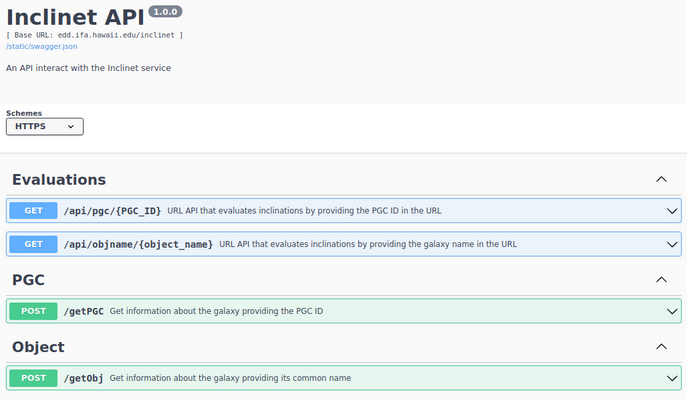
Fig. 22: Screenshot of the API documentation in the Swagger format: https://edd.ifa.hawaii.edu/inclinet/api/docs#/

1. URL query that reports all evaluated inclinations and other results in json format. <PGC_id> is the galaxy ID in the HyperLeda catalog.

$ curl http://edd.ifa.hawaii.edu/inclinet/api/pgc/<PGC_id>
 

• example:

  $ curl http://edd.ifa.hawaii.edu/inclinet/api/pgc/2557

  See Output ...

     {
     "status": "success",
     "galaxy": {
         "pgc": "2557",
         "ra": "10.6848 deg",
         "dec": "41.2689 deg",
         "fov": "266.74 arcmin",
         "pa": "35.0 deg",
         "objname": "NGC0224"
     },
     "inclinations": {
         "Group_0": {
         "model4": 69.0,
         "model41": 72.0,
         "model42": 76.0,
         "model43": 71.0
         },
         "Group_1": {
         "model5": 73.0,
         "model51": 73.0,
         "model52": 74.0,
         "model53": 74.0
         },
         "Group_2": {
         "model6": 73.0,
         "model61": 76.0,
         "model62": 76.0,
         "model63": 67.0
         },
         "summary": {
         "mean": 72.83333333333333,
         "median": 73.0,
         "stdev": 2.6718699236468995
         }
     },
     "rejection_likelihood": {
         "model4-binary": 50.396937131881714,
         "model5-binary": 20.49814760684967,
         "model6-binary": 65.37048816680908,
         "summary": {
         "mean": 45.42185763518015,
         "median": 50.396937131881714,
         "stdev": 18.65378065042258
         }
     }
     }

2. Given the galaxy common name, the following URL reports all evaluated inclinations and other results in json format. <obj_name> is the galaxy galaxy name. Galaxy name is looked up on NASA/IPAC Extragalactic Database and the corresponding PGC number would be used for the purpose of our analysis.

   $ curl http://edd.ifa.hawaii.edu/inclinet/api/objname/<obj_name>
   

• example:

     $ curl http://edd.ifa.hawaii.edu/inclinet/api/objname/M33

  See Output ...

     {
     "status": "success",
     "galaxy": {
         "pgc": 5818,
         "ra": "23.4621 deg",
         "dec": "30.6599 deg",
         "fov": "92.49 arcmin",
         "pa": "22.5 deg",
         "objname": "M33"
     },
     "inclinations": {
         "Group_0": {
         "model4": 54.0,
         "model41": 58.0,
         "model42": 54.0,
         "model43": 52.0
         },
         "Group_1": {
         "model5": 54.0,
         "model51": 55.0,
         "model52": 52.0,
         "model53": 55.0
         },
         "Group_2": {
         "model6": 56.0,
         "model61": 57.0,
         "model62": 55.0,
         "model63": 53.0
         },
         "summary": {
         "mean": 54.583333333333336,
         "median": 54.5,
         "stdev": 1.753963764987432
         }
     },
     "rejection_likelihood": {
         "model4-binary": 41.28798842430115,
         "model5-binary": 4.068140685558319,
         "model6-binary": 55.70455193519592,
         "summary": {
         "mean": 33.68689368168513,
         "median": 41.28798842430115,
         "stdev": 21.754880259382322
         }
     }
     }

3. Given the galaxy image, the following API call reports all evaluated inclinations and other results in json format.

$ curl -F 'file=@/path/to/image/galaxy.jpg' http://edd.ifa.hawaii.edu/inclinet/api/file

where /path/to/image/galaxy.jpg would be replaced by the name of the galaxy image. The accepted suffixes are 'PNG', 'JPG', 'JPEG', 'GIF' and uploaded files should be smaller than 1 MB.

• example:

     $ curl -F 'file=@/path/to/image/NGC_4579.jpg' http://edd.ifa.hawaii.edu/inclinet/api/file

  See Output ...

   ```bash
      {
      "status": "success",
      "filename": "NGC_4579.jpg",
      "inclinations": {
          "Group_0": {
          "model4": 47.0,
          "model41": 51.0,
          "model42": 50.0,
          "model43": 47.0
          },
          "Group_1": {
          "model5": 49.0,
          "model51": 49.0,
          "model52": 51.0,
          "model53": 52.0
          },
          "Group_2": {
          "model6": 50.0,
          "model61": 49.0,
          "model62": 49.0,
          "model63": 48.0
          },
          "summary": {
          "mean": 49.333333333333336,
          "median": 49.0,
          "stdev": 1.49071198499986
          }
      },
      "rejection_likelihood": {
          "model4-binary": 84.28281545639038,
          "model5-binary": 94.24970746040344,
          "model6-binary": 88.11054229736328,
          "summary": {
          "mean": 88.88102173805237,
          "median": 88.11054229736328,
          "stdev": 4.105278145778375
          }
      }
      }
   ```
  

7. Documentation

The full documentation of this application is available here.

8. Acknowledgments

8.1. About the data

All data exposed by the IncliNET project belongs to

• Cosmicflows-4 program
• Copyright (C) Cosmicflows
• Team - The Extragalactic Distance Database (EDD)

8.2. Citation

Please cite the following paper and the gitHub repository of this project.

• Cosmicflows-4: The Catalog of ∼10,000 Tully-Fisher Distances

@ARTICLE{2020ApJ...902..145K,
      author = {{Kourkchi}, Ehsan and {Tully}, R. Brent and {Eftekharzadeh}, Sarah and {Llop}, Jordan and {Courtois}, H{\'e}l{\`e}ne M. and {Guinet}, Daniel and {Dupuy}, Alexandra and {Neill}, James D. and {Seibert}, Mark and {Andrews}, Michael and {Chuang}, Juana and {Danesh}, Arash and {Gonzalez}, Randy and {Holthaus}, Alexandria and {Mokelke}, Amber and {Schoen}, Devin and {Urasaki}, Chase},
       title = "{Cosmicflows-4: The Catalog of {\ensuremath{\sim}}10,000 Tully-Fisher Distances}",
     journal = {\apj},
    keywords = {Galaxy distances, Spiral galaxies, Galaxy photometry, Hubble constant, H I line emission, Large-scale structure of the universe, Inclination, Sky surveys, Catalogs, Distance measure, Random Forests, 590, 1560, 611, 758, 690, 902, 780, 1464, 205, 395, 1935, Astrophysics - Astrophysics of Galaxies},
        year = 2020,
       month = oct,
      volume = {902},
      number = {2},
         eid = {145},
       pages = {145},
         doi = {10.3847/1538-4357/abb66b},
archivePrefix = {arXiv},
      eprint = {2009.00733},
primaryClass = {astro-ph.GA},
      adsurl = {https://ui.adsabs.harvard.edu/abs/2020ApJ...902..145K},
     adsnote = {Provided by the SAO/NASA Astrophysics Data System}
}

8.3. Author

• Ehsan Kourkchi - ekourkchi@gmail.com

8.4. Disclaimer

• All rights reserved. The material may not be used, reproduced or distributed, in whole or in part, without the prior agreement.

9. References

• Recovering the Structure and Dynamics of the Local Universe (Ph.D. Thesis by E. Kourkchi - 2020)
• Cosmicflows-4: The Catalog of ~10000 Tully-Fisher Distances (Journal ref: Kourkchi et al., 2020, ApJ, 902, 145, arXiv:2009.00733) refer to section 2.3
• Global Attenuation in Spiral Galaxies in Optical and Infrared Bands (Journal ref: Kourkchi et al.,2019, ApJ, 884, 82, arXiv:1909.01572) refer to section 2.5
• Galaxy Inclination Zoo (GIZ)
• GIZ help page
• GIZ Blog