Aman_Tasks_Sentinel_Data

Aman_Task1

Contents :

1. Tools Used And Data
2. Steps Executed
3. Uses
4. References

Tools Used and Data

• Jupyter Notebook - I mostly work on PyCharm but packages like Shapely and KeplerGL works better on Jupyter Notebook. The GIS Virtual Env was already ready with me.
• QGIS - For viewing and perform some operations on the Data
• GitHub - Version Control
• Data - Area of Interest Data was downloaded from the Google Driver [1] in GeoJSON format

Steps Executed Data Preprocessing

(Please open the file Task1_ClippingSentinel2Data.ipynb)

1. I processed the GeoJSON data in Jupyter Notebook. (data\remote_sensing_challenge_AOI.geojson)

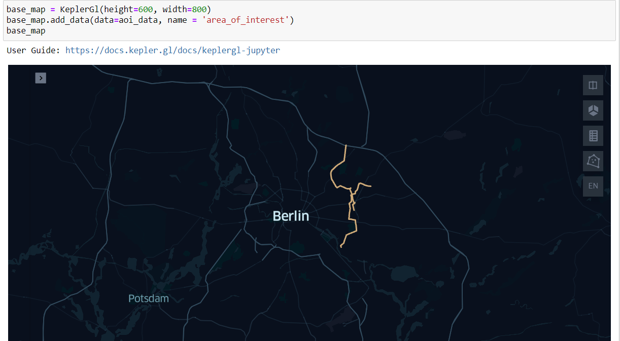
2. Using Kepler GL, I found the AreaofInterest is North Eastern Part of Berlin, Germany. Picture can be found here or from images\Task1_KeplerGLLocationDetection.png

3. I was downloading the data from USGS Gov Website [2], but the partnership between ESA and the USGS allows only for the distribution of Level-1C. As per the Task we need Level 2-A Data.

4. Finally, I downloaded the data from Copernicus Open Access Hub [3] with the following properties :

   • Selected the Berlin Location
   • In the advanced search I selected Mission - Sentinel 2
   • Product Type as S2MSI2A
   • Year 2020
   • (Through this I was able to download the correct data with the requirement - Sentinel-2 level 2A tile from any practical TOI (2019 or 2020)

5. I selected the 12 (Total 13, but removed 10 - cirrus band which gives no ground information) specific bands which are needed and put them in the folder data\13bands from the .SAFE folder data structure downloaded from Copernicus Access Hub. I refered the information of the Sentinel 2 bands from Wikipedia [4]

6. I selected the SCL Layer (20m), and opened it in SQIS to make the NO_DATA,SATURATED_OR_DEFECTIVE, CLOUD_HIGH_PROBABILITY as NOVALUE, (In QGIS, we get an option to set the No Data Values when saving the Raster Layer) and saved the new file as data\13bands\scllayer_nodata_band.tif . The label for each classification I found from the Sentinel [5] Website

7. I opened those 13 Bands (12 + 1 SCL) in the QGIS and created a Virtual Layer.

8. There was a color mismatch so I edited the virtual layer and set the BGR (Bands 2,3,4 respectively), and I was able to see an observable satellite map of Berlin (And its surroundings). I got the information of the bands from SatimagingCorp [6] website.

9. I could see the Satellite images have an EPSG of 32633, hence I created a new AOI with EPSG 32633 with the name as data\remote_sensing_challenge_AOI32633.geojson

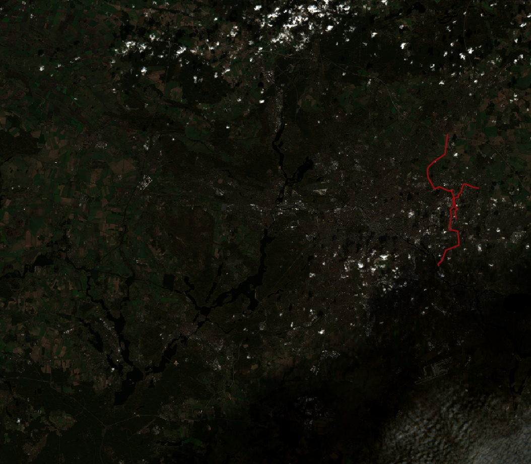
10. Just to validate the Correct data has been downloaded, I verified by adding the AOI on top of the layer, and the image can be seen here or from images\Task1_satellite_aoi_validate.png

11. All the bands (12 + SCL with NOVALUE for 3 parameter) were merged into a GeoTIFF. (data\mergedBandswithSCL.tif), which will serve as the input for the clipping in the jupyer notebook.

12. I clipped the input of the mergedBandswithSCL.tif which can be found in the Task1_ClippingSentinel2Data.ipynb file.

13. The Final Output can be seen below (With the AOI) or in the file images\task1_clipped_output.png and the final clipped GeoTIFF will be found in data\clippedGeoTIFF.tif

Uses

Data Clipping - As the data from Satellite Hubs which gets downloaded are far enormous than the Area of Interest, thus clipping helps us to trim the map (data) which only contains the information of and around the Area of Interest. The clipped data is considerably less in size and eventually helps to process any operation on the clipped data faster.

References

• [1] https://drive.google.com/file/d/1cYulst52qOsx1VOOtVQo5sRdUugYqEpl/view
• [2] https://www.usgs.gov/centers/eros/science/usgs-eros-archive-sentinel-2?qt-science_center_objects=0#qt-science_center_objects
• [3] https://scihub.copernicus.eu/dhus/#/home
• [4] https://en.wikipedia.org/wiki/Sentinel-2#Spectral_bands
• [5] https://sentinel.esa.int/web/sentinel/technical-guides/sentinel-2-msi/level-2a/algorithm
• [6] https://www.satimagingcorp.com/satellite-sensors/other-satellite-sensors/sentinel-2a/ a

Aman_Task_2

Contents :

1. Tools Used And Data
2. FileNames Legend
3. Steps Executed
   • Common Task
   • Sub - Task 1
   • Sub - Task 2
   • Sub - Task 3
4. Uses
5. References

Tools Used And Data

• PyCharm IDE - As this task has less of interim image displays, I worked on PyCharm as I am more comfortable in that.
• GitHub - Version Control
• Data - TIF File - Converted to JPG of the Task 1 Output. data\Task2_Image.jpg
• Magick - To Convert the images into GIF

FileNames Legend

• FD - Feature Detection
• ED - Edge Detection
• LPF - Low Pass Filter
• util - Utility Class

Steps Executed

Common Task

1. I created a util class to read the file (Colour and Grey format) and to write the image on the disk. (Util class will be used in all 3 SubTasks). Methods created are readFile_coloured(), readFile_gray() and writeImage().

SubTask 1

(Please open the file Task2_1_FeatureDetection.py)

1. I used two algorithms for the Feature Detection. SIFT and ORB.

2. Feature Detection using Convolutional neural network would really be beneficial [1], but due to lack of time I have used the Computer Vision module CV2.

3. I read about SIRF [2] and about the Feature Detection Algorithms of CV module [3]

4. I used the SIFT and ORB Feature Detection Algorithms on the Image, and saved the output. images\Task2_1_FB_GreyOriginialImage.jpg, images\Task2_1_FB_SIFT.jpg and images\Task2_1_FB_ORB.jpg. I had overridden the nfeatures for both the algorithms and set the flag as DRAW_MATCHES_FLAGS_DRAW_RICH_KEYPOINTS, which will draw a circle with size of keypoint and even show its orientation. A combined image of all three is also stored in images\Task2_1_FB_CombinedImage.jpeg, and also displayed below.

5. In future we can also use a label marker. [4]

SubTask 2

(Please open the file Task2_2_EdgeDetection.py)

1. For Edge Detection, I used Canny [5], Laplacian and Sobel Algorithms [6]

2. I have stored all the images images\Task2_2_ED_GreyOriginalImage.jpg, images\Task2_2_ED_Canny.jpg, images\Task2_2_ED_Laplacian.jpg, images\Task2_2_ED_SobelX.jpg, images\Task2_2_ED_SobelY.jpg, images\Task2_2_ED_SobelCombined.jpg. A combined image can be seen below or in images\Task2_2_ED_CombinedImage.jpeg. In addition to these I have also create a gif to see all the Edge Pattern in one transition images\Task2_2_ED_CombinedGIF.

Note :

1. 2_ED_Laplacian is not being displayed correctly in the combined file, please open the individual file image\Task2_2_ED_Laplacian.jpg to see the correct Edge Pattern
2. Blurring an image before Edge Detection is optional, but since it has a different task I have done that in Task2_3

SubTask 3

(Please open the file Task2_3_LowPassFilter.py)

1. I first read about the filter from the medium article [7], freeCodeCamp.org Youtube channel [8], the OpenCV API Documentation [9] and a mathematical explanation on the blog [10]

2. I used, filter2D, blur and GaussianBlur Image blurring techniques, and for filter2D I created two Kernels -> (5,5) and (3,3)

3. The outputs of each Image blurring techniques are stored in the images\Task2_3_LPF_Blur, images\Task2_3_LPF_Gassian_Blur, images\Task2_3_LPF_Convolved3, images\Task2_3_LPF_Convolved5, and the combined image in the images\Task2_3_LPF_AllFiltersCombined, and can be seen below.

Uses

1. Feature Detection - In the world of Geospatial, when we are dealing with a lot of Earth Observation Data, with feature detection we can detect Vehicles, Buildings, Vegetations, and a lot of structures which can be widely used in Military, Civil Engineering, Urban planning and more. Along with proper labelling techniques, we can also label and get to know the number of structures, number of vehicles and more in a given EO data.
2. Edge Detection - I believe, Edge Detection can be used to detect the size of the structures like a huge Vegetation Land, a Lake, a huge mall and more. Edge detection can also let us know how dense a particular area is with structures.
3. Low Pass Filter - Running a Low Pass Filter or blurring the image removes the high frequency details and makes the image more smooth by averaging the pixels. I believe this might be useful to extract large structures in the image.

References

• [1] TY - JOUR AU - Hoeser, Thorsten AU - Bachofer, Felix AU - Kuenzer, Claudia PY - 2020/09/18 SP - 3053 T1 - Object Detection and Image Segmentation with Deep Learning on Earth Observation Data: A Review-Part II: Applications VL - 12 DO - 10.3390/rs12183053 JO - Remote Sensing ER - https://www.researchgate.net/publication/344298612_Object_Detection_and_Image_Segmentation_with_Deep_Learning_on_Earth_Observation_Data_A_Review-Part_II_Applications

• [2] Author:Niklas NilssonSupervisors:Villiam Aspegren, Carmenta Geospatial TechnologiesHaidar Al-Naseri, Dep. of Physics, Umeå UniversityExaminer: Eddie Wadbro, Dep. of Computer Science, Umeå Univeristy - extension://bfdogplmndidlpjfhoijckpakkdjkkil/pdf/viewer.html?file=http%3A%2F%2Fwww.diva-portal.org%2Fsmash%2Fget%2Fdiva2%3A1321511%2FFULLTEXT02.pdf

• [3] https://docs.opencv.org/3.4/db/d27/tutorial_py_table_of_contents_feature2d.html

• [4] https://github.com/developmentseed/label-maker/tree/master/examples

• [5] https://docs.opencv.org/3.4/da/d22/tutorial_py_canny.html

• [6] https://www.bogotobogo.com/python/OpenCV_Python/python_opencv3_Image_Gradient_Sobel_Laplacian_Derivatives_Edge_Detection.php

• [7] https://medium.com/nattadet-c/image-filters-41c23f09c600

• [8] https://www.youtube.com/watch?v=oXlwWbU8l2o

• [9] https://docs.opencv.org/3.4/d4/d86/group__imgproc__filter.html

• [10] https://cdn.diffractionlimited.com/help/maximdl/Low-Pass_Filtering.htm