This one uses the NARX model to predict the forthcoming house price in months of 2017.
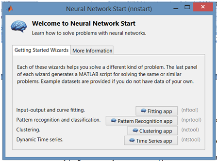
To execute this code run main.m in MATLAB. It will open a GUI and proceed further as desire.
To predict the house price, we need a dataset which can train the neural network. This dataset must be large enough to train the network so that overfitting of results can be avoided. We have used the dataset obtained from London data store. it contains the data form year 1995-2015. This is categorised as • ID (Transaction ID) • Date (Date processed, Month of transaction, Year of transaction, etc) • Transaction Price • Property classification (Type, Build, Tenure) • Address information (Postcode, Local authority, Full address, Borough, Ward, etc) These variables are further divided as dependent variables and independent variables for the NN training. Out of these dependent variables will be the input for training and independent variable will act as target. The table of these variables is given as
| Dependent variables | Independent Variables |
|---|---|
| 1. Date of transaction (Month, Year) | Price of property (£) |
| 2.Type(Detached/Semidetached/Terrace/Flat) | |
| 3. Build (Old/New) | |
| 4. Tenure (Leasehold/Freehold) |
The data given is not statistical data but for the NN toolbox to feed, we need the data in that form so , we converted data into statistical format. • the month/year of transaction is converted into decimal number series by using a MATLAB function 'datenum' .
example: datenum('01/05/2017')
ans =
736700
• property of four types in the data as shown in the table, we assigned decimal values to those as: Detached (D)=1 Semi-detached (S)=2 Terrace (T) =3 Flat (F)=4
• Build new (N)=1 Old (Y) =2
• Tenure Leasehold(L)=1 FreeHold (F) =2
The dataset is very large and MATLAB can't handle this much dataset, so we used the dataset form only 2013-2015 and predicted the house price for 2016 first and used that to along with rest to predict the 2017 year house price.
The downloaded data is in csv format, so we converted that into .mat format first by importing the data into MATLAB import toolbox and then save as .mat file. We followed this process as importing the data form .csv file will take more time than .mat.
After data is loaded into script and assigned into corresponding variables, these values are normalised to reduce the difference in between all input and output values to NN. This way the similarity of data can be increased and accuracy of predicted price.
After NN is trained, a model is ready with us which will be used for predicting next year or next quarter year house price. No input and output of time series to be predicted is available with us. So we will use the recent year's known values equal to hidden layers number and predfixed to days price to be predicted. For example in a quarter of 90 days, 20 days data from previous known year is added prior to these 90 days matrix whose these 90 elements will be zero. This data will be further used to predict the required time frame house price.
% daysahead=30;

[xs,xis,ais,ts] = preparets(nets,X(end:-1:end-daysahead-numel(inputDelays)+1)...
                               ,{},T(end:-1:end-daysahead-numel(inputDelays)+1));
ys = nets(xs,xis,ais);
predictedop=cell2mat(ys);
predictedop=predictedop.*max(price1);
The function 'preparets' makes the data usable for NN training. This code snippet gives us the predicted output which is further plotted and compared in our GUI with previous year house price of same quarter.
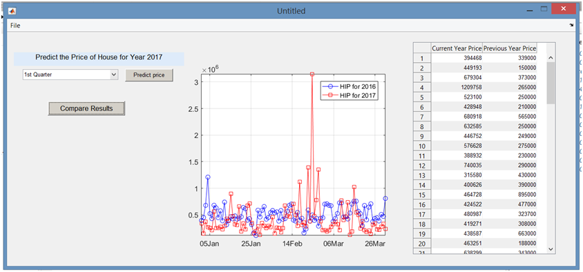 Figure 1.3.1: our designed GUI for predicting the house price of each quarter
MATLAB also make it possible to write the respective month on X-axis in the plot as in above figure. The trained network's accuracy can be judged by plotting a curve of MSE and iterations required as shown in figure 1.3.2. This is also a convergence curve, as soon as MSE settles to lowest value, good is the NN training. In our work error is settled at 10-4 which is desired.
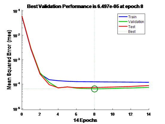
figure 1.3.2: MSE vs Iteration plot after NN traininig
'trainlm' is the function which is based on Laquanberg method for the backpropagation method. A feedback network is generated with two time stamp delay and 20 neurons in an hidden layer in our work.