GerryChain-Templates

This repo provides an evolving set of instructional guides for using the GerryChain package for generating dual graph partitions. More detailed technical documentation can be found here and my introduction to the mathematics of Markov chains and MCMC for redistrcitng can be found here: (pdf) (webpage) (GitHub).

Overview

These templates assume that you have already installed GerryChain (see here or here for directions) and are ready to start building your own ensembles. Since some of the examples use real-world data, you should clone this repo to your computer - this will also make it easy to get access to updates to the templates. Once you have downloaded everything you should be able to run the templates individually by navigating to the appropriate subfolder and entering:

python grid_chain_simple.py

Here are links to the current templates:

• Grids
• grid_chain_simple.py
• grid_chain_medium.py
• grid_chain_complicated.py
• Pennsylvania
• PA_Chain.py
• Alaska
• AK_Chain.py

More details about the contents of these files are provided below the simple grids example.

Grids are fun!

The best place to start is with the simple grids example. This template breaks the code into pieces, building the graph and partition components separately before doing a couple of small runs to compare ReCom to Flip. We start by importing the packages we need:

import os
import random
import json
import geopandas as gpd
import functools
import datetime
import matplotlib
#matplotlib.use('Agg')
import matplotlib.pyplot as plt
import numpy as np
import csv
from networkx.readwrite import json_graph
import math
from functools import partial
import networkx as nx
import numpy as np


from gerrychain import Graph
from gerrychain import MarkovChain
from gerrychain.constraints import (Validator, single_flip_contiguous,
within_percent_of_ideal_population, UpperBound)
from gerrychain.proposals import propose_random_flip, propose_chunk_flip
from gerrychain.accept import always_accept
from gerrychain.updaters import Election,Tally,cut_edges
from gerrychain import GeographicPartition
from gerrychain.partition import Partition
from gerrychain.proposals import recom
from gerrychain.metrics import mean_median, efficiency_gap

Next we build a gn x k by gn x k graph split into k vertical columns:

#BUILD GRAPH

gn=6
k=5
ns=50
p=.5

graph=nx.grid_graph([k*gn,k*gn])



for n in graph.nodes():
    graph.node[n]["population"]=1


    if random.random()<p:
        graph.node[n]["pink"]=1
        graph.node[n]["purple"]=0
    else:
        graph.node[n]["pink"]=0
        graph.node[n]["purple"]=1
    if 0 in n or k*gn-1 in n:
        graph.node[n]["boundary_node"]=True
        graph.node[n]["boundary_perim"]=1

    else:
        graph.node[n]["boundary_node"]=False

#this part adds queen adjacency
#for i in range(k*gn-1):
#    for j in range(k*gn):
#        if j<(k*gn-1):
#            graph.add_edge((i,j),(i+1,j+1))
#            graph[(i,j)][(i+1,j+1)]["shared_perim"]=0
#        if j >0:
#            graph.add_edge((i,j),(i+1,j-1))
#            graph[(i,j)][(i+1,j-1)]["shared_perim"]=0



########## BUILD ASSIGNMENT
cddict = {x: int(x[0]/gn)  for x in graph.nodes()}

######PLOT GRIDS

plt.figure()
nx.draw(graph, pos = {x:x for x in graph.nodes()} ,node_size = ns, node_shape ='s')
plt.show()

cdict = {1:'pink',0:'purple'}

plt.figure()
nx.draw(graph, pos = {x:x for x in graph.nodes()}, node_color = [cdict[graph.node[x]["pink"]] for x in graph.nodes()],node_size = ns, node_shape ='s' )
plt.show()

plt.figure()
nx.draw(graph, pos = {x:x for x in graph.nodes()}, node_color = [cddict[x] for x in graph.nodes()] ,node_size = ns, node_shape ='s',cmap = 'tab20')
plt.show()

Original Graph	Random Vote Data	Initial Partition

Next we configure the partitions, updaters, and constraints.

####CONFIGURE UPDATERS

def step_num(partition):
    parent = partition.parent

    if not parent:
        return 0


    return parent["step_num"] + 1

updaters = {'population': Tally('population'),
                    'cut_edges': cut_edges,
                    'step_num': step_num,
                    "Pink-Purple": Election("Pink-Purple", {"Pink":"pink","Purple":"purple"})}



#########BUILD PARTITION

grid_partition = Partition(graph,assignment=cddict,updaters=updaters)

#ADD CONSTRAINTS
popbound=within_percent_of_ideal_population(grid_partition,.1)

#########Setup Proposal
ideal_population = sum(grid_partition["population"].values()) / len(grid_partition)

tree_proposal = partial(recom,
                       pop_col="population",
                       pop_target=ideal_population,
                       epsilon=0.05,
                       node_repeats=1
                      )

#######BUILD MARKOV CHAINS


recom_chain=MarkovChain(tree_proposal, Validator([popbound]),accept=always_accept,
initial_state=grid_partition, total_steps=100)

boundary_chain=MarkovChain(propose_random_flip, Validator([single_flip_contiguous, popbound]),accept=always_accept,
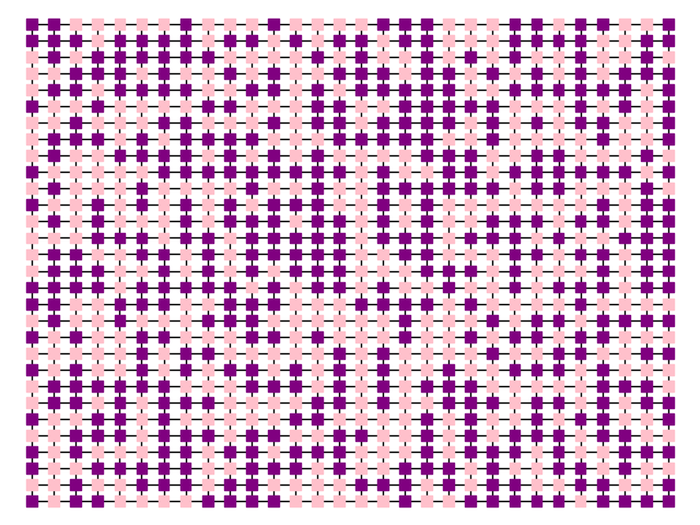
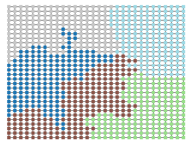
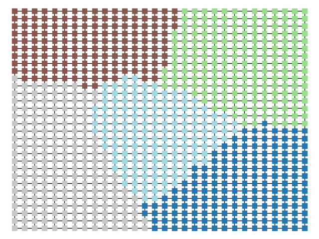
initial_state=grid_partition, total_steps=10000)

Finally, we run two chains, one with each proposal method, and record a variety of statistics. The final state of each of the two chains will be displayed. Notice that even though the ReCom chain only takes 100 steps, it travels much further than the 10,000 step boundary chain.

#########Run MARKOV CHAINS

rsw = []
rmm = []
reg = []
rce = []

for part in recom_chain:
    rsw.append(part["Pink-Purple"].wins("Pink"))
    rmm.append(mean_median(part["Pink-Purple"]))
    reg.append(efficiency_gap(part["Pink-Purple"]))
    rce.append(len(part["cut_edges"]))
    """
    plt.figure()
    nx.draw(graph, pos = {x:x for x in graph.nodes()}, node_color = [dict(part.assignment)[x] for x in graph.nodes()] ,node_size = ns, node_shape ='s',cmap = 'tab20')
    plt.savefig(f"./Figures/recom_{part['step_num']:02d}.png")
    plt.close()
    """

plt.figure()
nx.draw(graph, pos = {x:x for x in graph.nodes()}, node_color = [dict(part.assignment)[x] for x in graph.nodes()] ,node_size = ns, node_shape ='s',cmap = 'tab20')
plt.show()


bsw = []
bmm = []
beg = []
bce = []

for part in boundary_chain:
    bsw.append(part["Pink-Purple"].wins("Pink"))
    bmm.append(mean_median(part["Pink-Purple"]))
    beg.append(efficiency_gap(part["Pink-Purple"]))
    bce.append(len(part["cut_edges"]))
    """
    plt.figure()
    nx.draw(graph, pos = {x:x for x in graph.nodes()}, node_color = [dict(part.assignment)[x] for x in graph.nodes()] ,node_size = ns, node_shape ='s',cmap = 'tab20')
    plt.savefig(f"./Figures/boundary_{part['step_num']:04d}.png")
    plt.close()
    """

plt.figure()
nx.draw(graph, pos = {x:x for x in graph.nodes()}, node_color = [dict(part.assignment)[x] for x in graph.nodes()] ,node_size = ns, node_shape ='s',cmap = 'tab20')
plt.show()

ReCom Ensemble	Boundary Ensemble

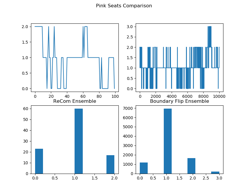
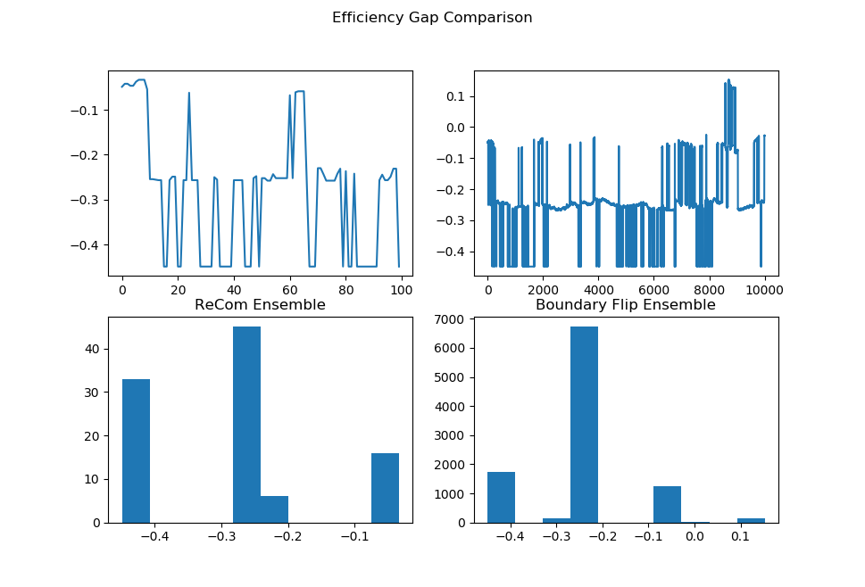
After the chain runs, we make some plots comparing the behavior of the ensembles.

##################Partisan Plots

names = ["Cut Edges", "Mean Median", "Pink Seats", "Efficiency Gap"]
lists = [[rce, bce], [rmm, bmm], [rsw, bsw], [reg, beg]]


for z in range(4):
    plt.figure()
    plt.suptitle(f"{names[z]} Comparison")

    plt.subplot(2, 2, 1)
    plt.plot(lists[z][0])



    plt.subplot(2, 2, 3)
    plt.hist(lists[z][0])
    plt.title("ReCom Ensemble")


    plt.subplot(2, 2, 2)
    plt.plot(lists[z][1])

    plt.subplot(2, 2, 4)
    plt.hist(lists[z][1])
    plt.title("Boundary Flip Ensemble")
    fig = plt.gcf()
    fig.set_size_inches((8,7))
    plt.show()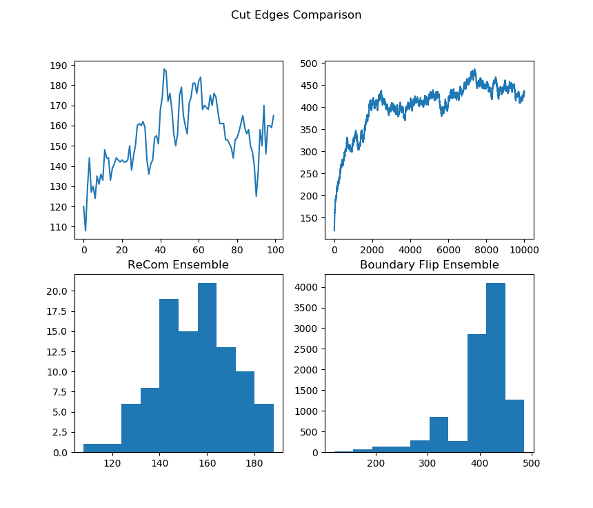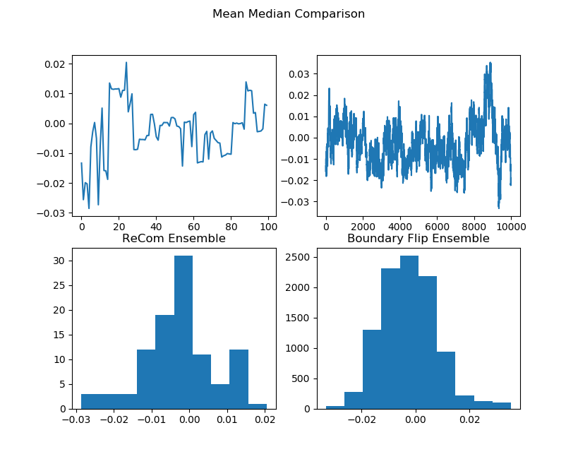

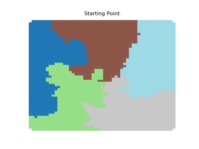
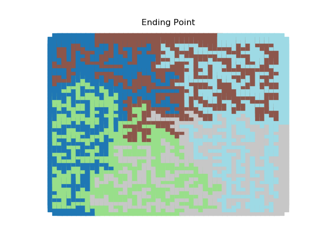
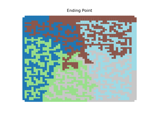
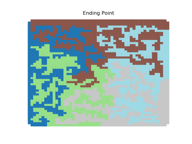
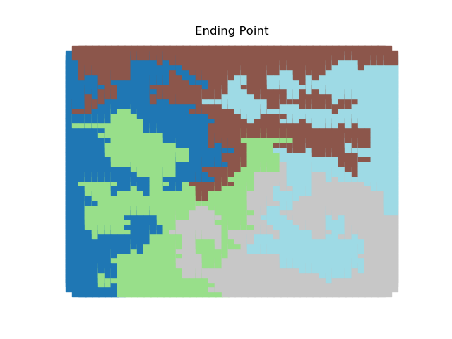
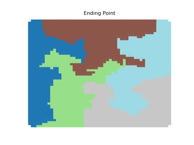
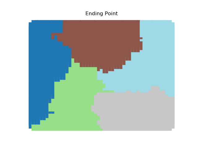
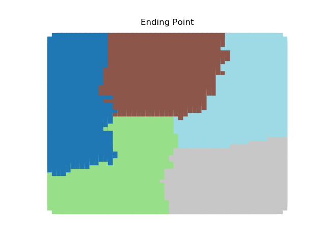
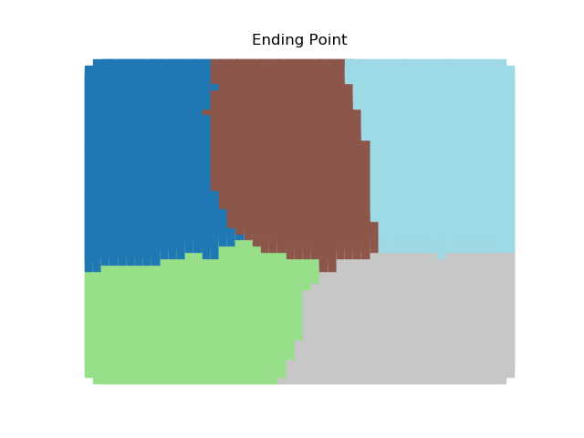
More Grids

The two other grid chains use more complicated tools to generate districting plans with short boundary lengths. Both examples start by using a short (100 step) ReCom run to turn the initial vertical stripes partition into a random starting point. Then, they use a longer (10,000 step) boundary flip proposal to generate a very wiggly districting plan with lots of tentacles. To generate nicer looking final plans, the medium chain uses a spectral clustering Recom step:

Initial Partition	Short Recom	Long Boundary	Spectral Cleanup

while the complicated chain uses simulated annealing on the boundary proposal. The target distribution is proportional to a base x raised to the negative boundary length multiplied by the inverse temperature. This chain runs significantly longer, the first 100k steps use the regular boundary walk (corresponding to an inverse temperature of zero). It then begins the annealing process, over the next 300k steps it linearly interpolates the inverse temperature from 0 to 3, and then spends the final 100k steps at 3. The figures below show the evolution of the chain as well as a heatmap of the number of times each node is flipped and the boundary length values. The code is currently configured to try this experiment with three different exponential bases (.1,2,4) and three different population tolerances (5%, 10%, 50%) to get a better sense for how these constraints interact.

Initial Partition	Short Recom	50k boundary steps	100k boundary steps
150 k boundary steps	200k boundary steps	250k boundary steps	300k boundary steps
400 k boundary steps	500k boundary steps	Flipped Nodes	Boundary length

Alaska

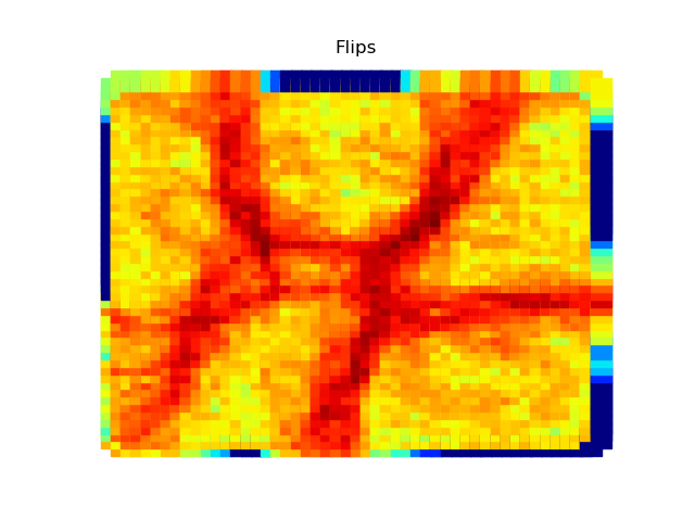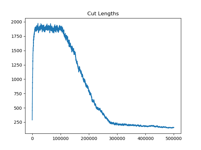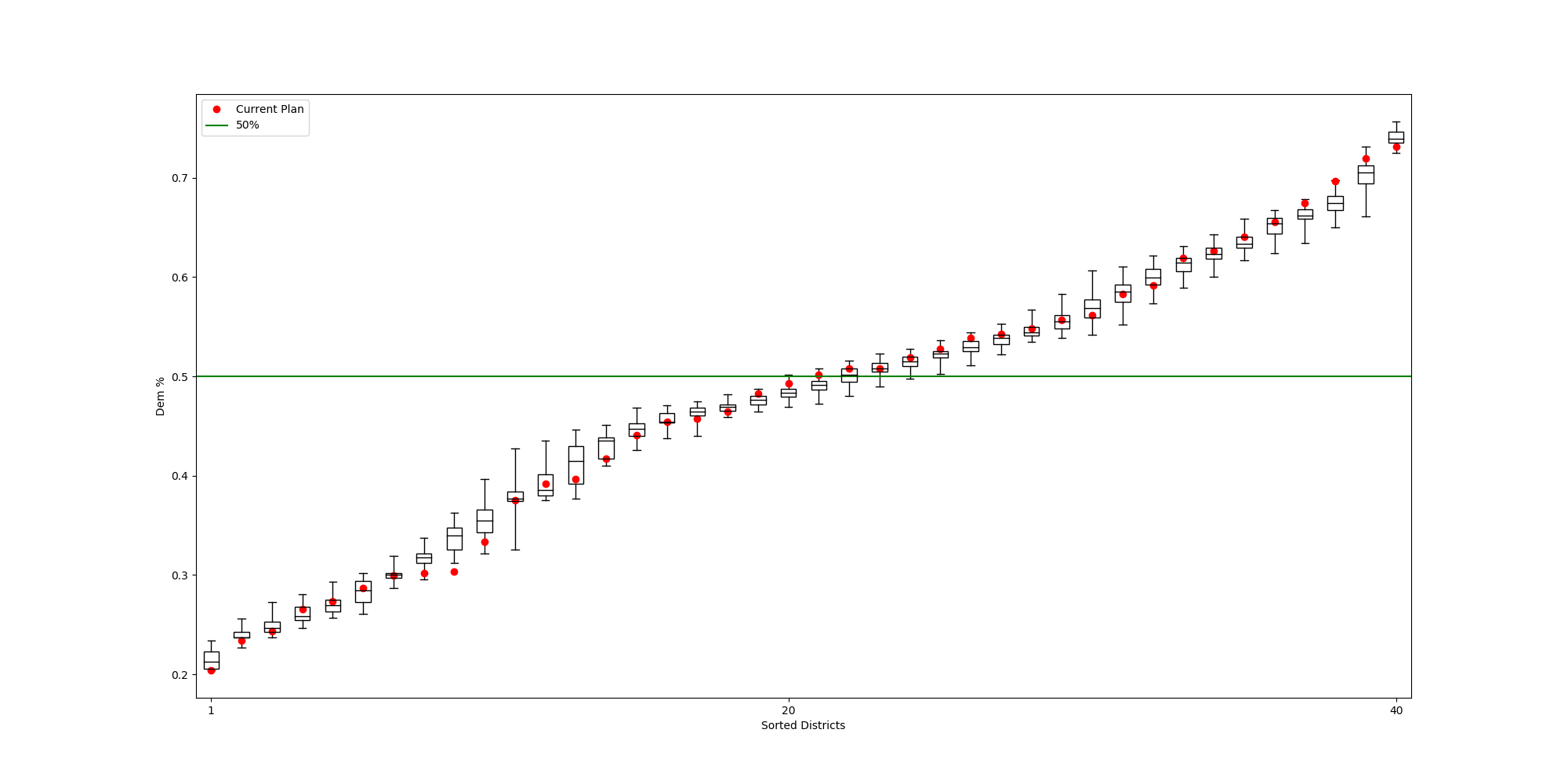
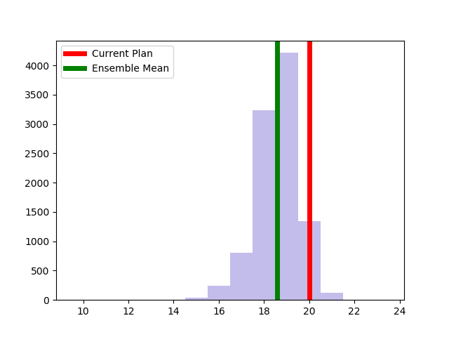
The Alaksa chain reproduces some of the experiments that were carried out in this paper. It begins by constructing a dual graph for the state directly from the shapefile and then adds in some extra edges to the dual graph to connect some islands and deletes some spurious edges that cross the water around Anchorage. The chain run itself is a pretty standard ReCom setup with a population constraint and a boundary length constraint. The only additional feature here is that at each step of the chain, the FKT algortithm is used to enumerate the number of perfect matchings of the current plat (i.e. the number of possible Senate pairings). After the run finishes, it provides box plots and seats histograms for four different election data sets as well as the proportion of Native populations in each district. These plots are automatically written to file with some summary values and .json files containing the underlying data.

Democratic %	House Seats	Competitive Districts	Number of Matchings

Pennsylvania

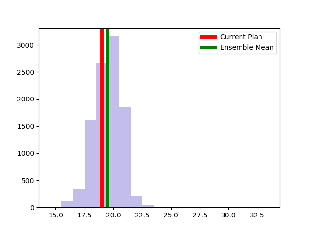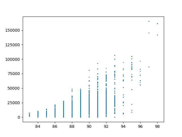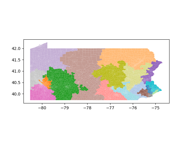
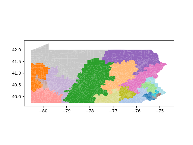
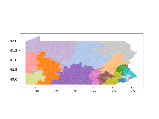
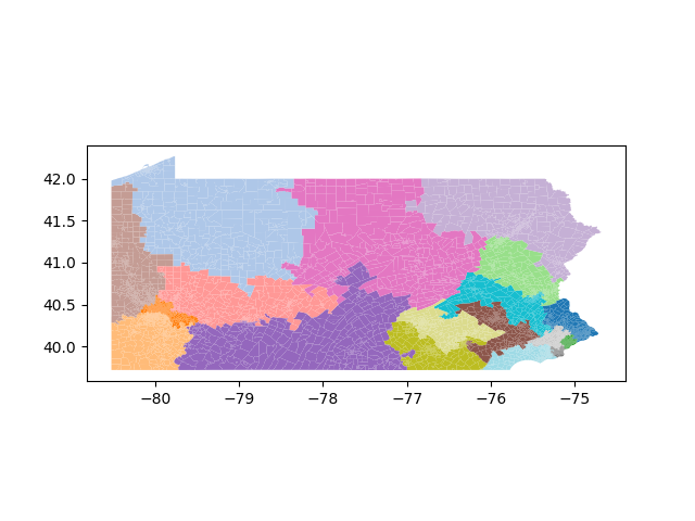
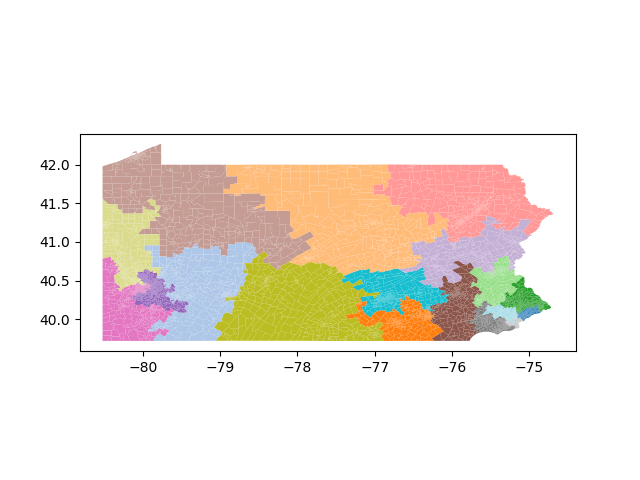
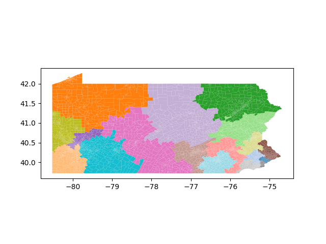
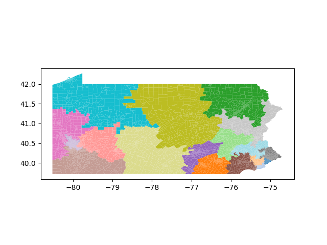
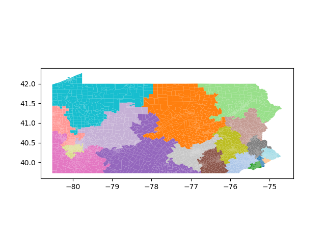
The Pennsylvania example explores a different approach to data processing. Here the dual graph is built directly from a .json file and no modifications are needed to make it contiguous. We start with the plan that was enacted in 2011 and take 1,000 ReCom steps while recording partisan statistics for 14 different elections. Every 100 steps, these values are written to file, along with a lot of the current plan. Once the chain has finished, the additional python file in the directory reads in the various outputs and creates box plots, traces, and histograms for each of the elections, as well as the boundary length, number of county splits, and population deviation. We have found this approach very useful for long runs, say 1,000,000 steps writing to file every 10,000 or so seems to keep the overhead RAM usage in a reasonable range.

Snapshot 1	Snapshot 2	Snapshot 3	Snapshot 4
Snapshot 5	Snapshot 6	Snapshot 7	Snapshot 8
Snapshot 9	Snapshot 10	Boundary Trace	Boundary Histogram
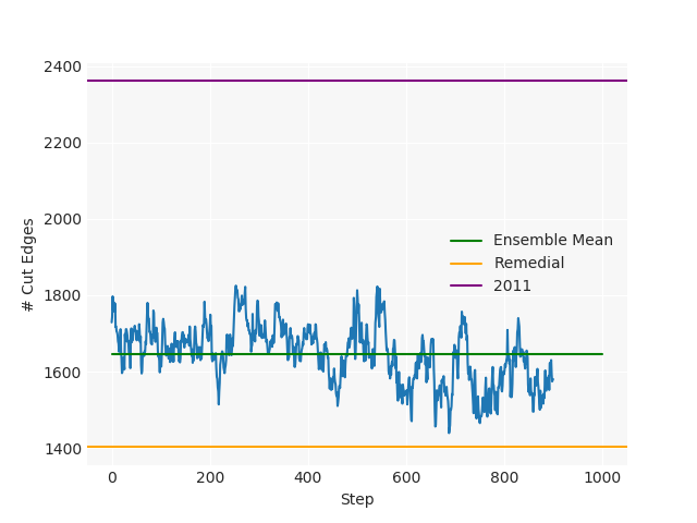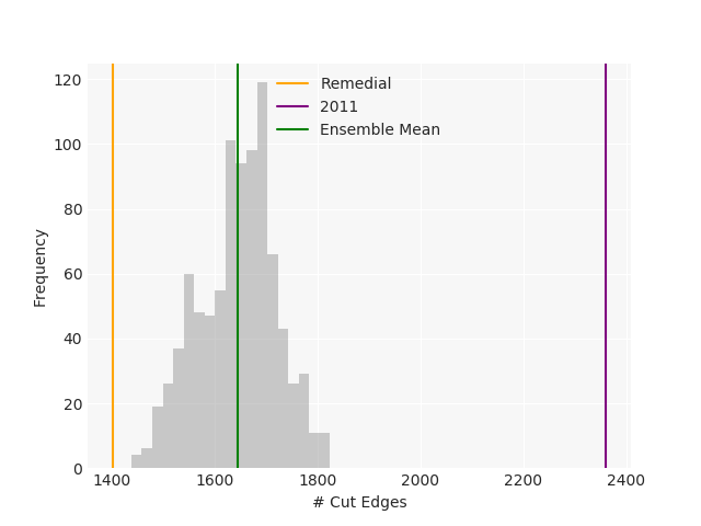Democratic %		Seats trace	Seats histogram
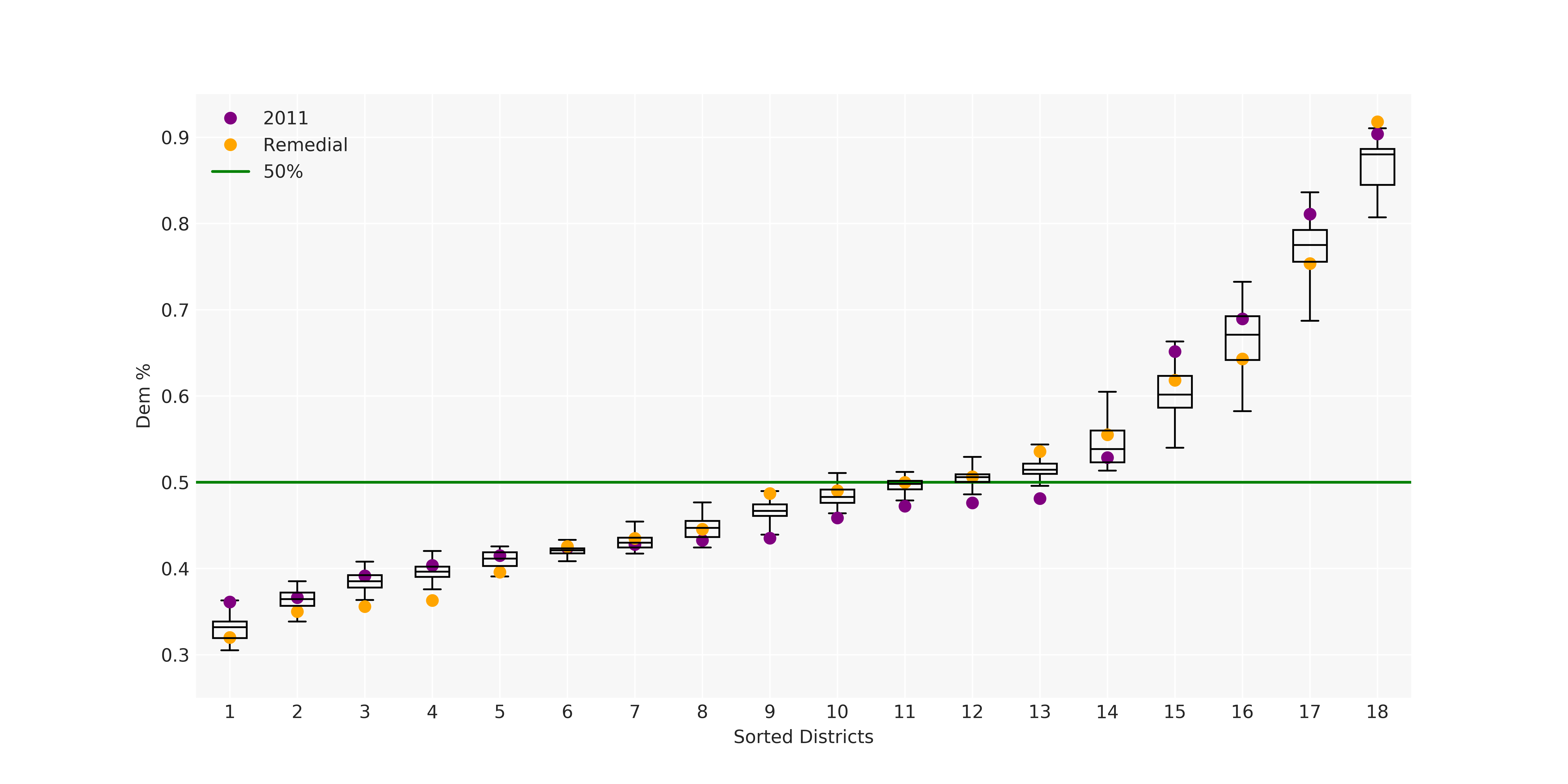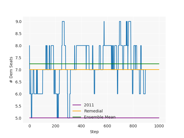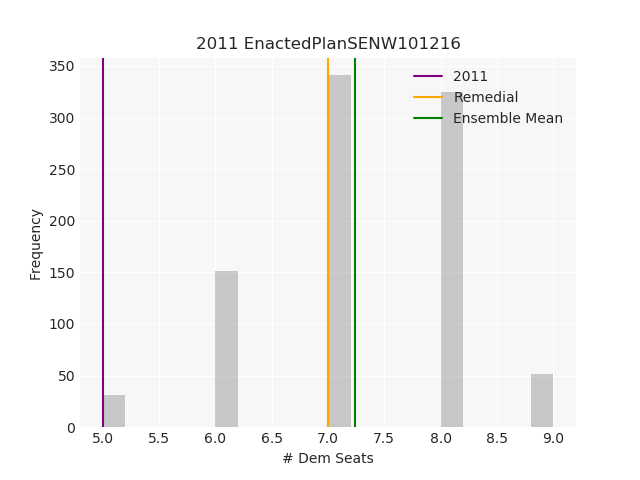Mean Median trace	Mean Median histogram	Efficiency Gap trace	Efficiency Gap histogram
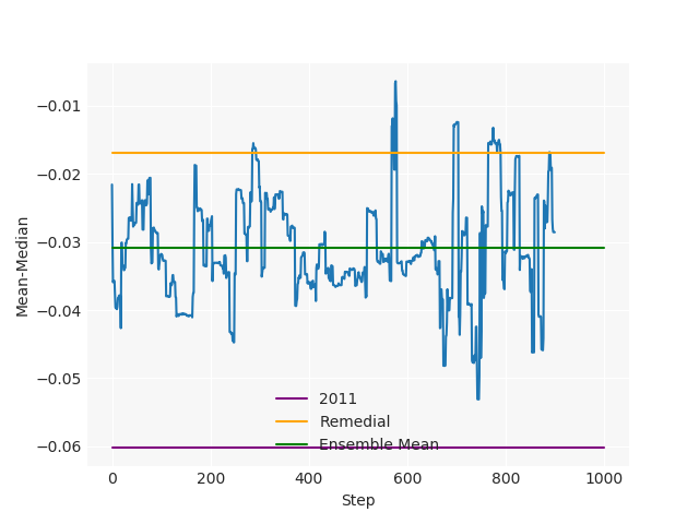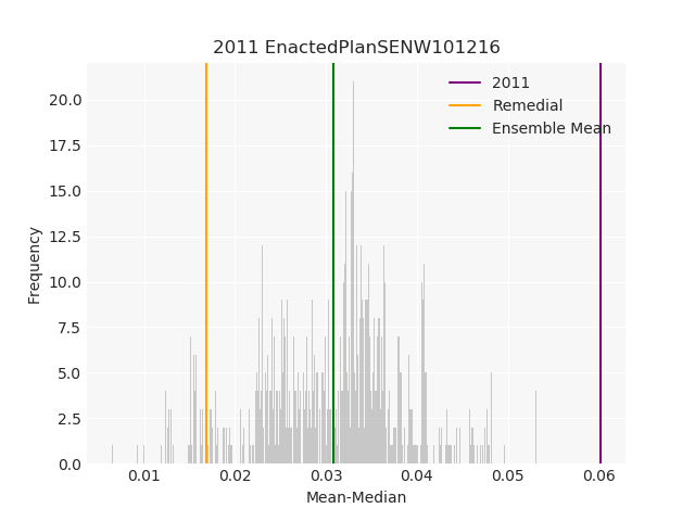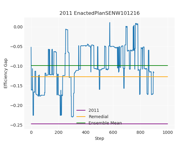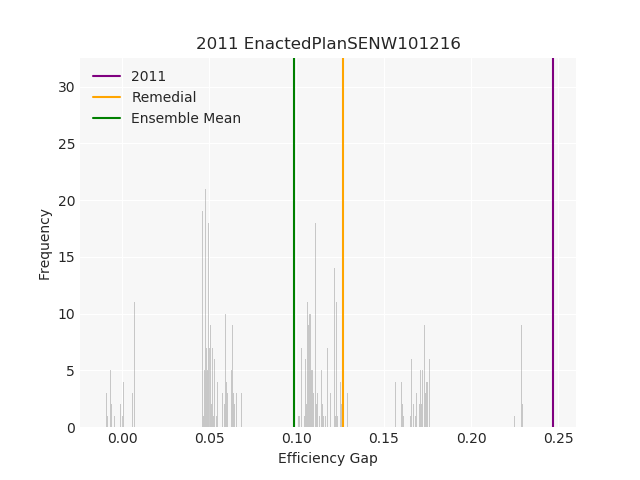