Image-to-image translation is a class of vision and graphics problems where the goal is to learn the mapping between an input image and an output image using a training set of aligned image pairs. [1] Neural Style Transfer is one way to perform image-to-image translation, which synthesizes a novel image by combining the content of one image with the style of another image-based on matching the Gram matrix statistics of pre-trained deep features [2]. Unlike recent work on "neural style transfer", we used CycleGAN [3] method which learns to mimic the style of an entire collection of artworks, rather than transferring the style of a single selecterd piece of art. Therefore, we can learn to generate photos in the style of, e.g., Van Gogh, rather than just in the style of Starry Night.
The dataset used for this project is sourced from a UC Berkley CycleGAN Directory and is downloaded from byTensorFlow Datasets. It consists of 8,000+ images from 2 classes: French Impressionist paintings and modern photography both of landscapes and other natural scenes. The size of the dataset for each artist/style was 526, 1073, 400, and 463 for Cezanne, Monet, Van Gigh, and Ukiyo-e.
In CycleGAN, there is no paired data to train on, so there is no guarantee that the input and the target pair
are meaningful during training. Thus, in order to enforce that the network learns the correct mapping, the cycle-consistency loss is used. In addition, adversarial loss is used to train generator and discriminator networks. Moreover, the identity loss is used to make sure generators generate the same image if the input image belongs to their target domain.
The objective of adversarial losses for the mapping function and its discriminator
is expressed as:
In the above formula, generator tries to minimize the
and in fact is trained to maximize the
while the discriminator
is trained to maximize the entire
.
On other hand, the same loss is applied for mapping from and its discriminator
:
Therefore, the total Adverserial loss is expressed as:
+
The goal is to generate images that are similar in style to the target domain while distinguising between the test data and the training data.
Adversarial losses alone do not guarantee that the content will preserved as it is mapped from the input to the target domain; therefore, cycle-consistent functions are implemented in order to prevent the learned mappings from contradicting each other. To calculate the cyclic loss, we measure the L1 distance (MAE) between the reconstructed image from the cycle and the truth image. This cycle consistency loss objective is:
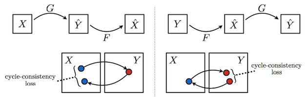
Figure 1: The CycleGAN model [3] contains two mapping functions and
, and associated adversarial discriminators
and
.
encourages
to translate
in to outputs indistinguishable from domain
and vice versa for
and
.
For painting to photo, it is helpful to introduce an additional loss to encourage the mapping to preserve color composition between the input and output. In particular, Identity loss regularizes the generator to be near an identity mapping when real samples of the target domain are provided as the input to the generator. The weight for the identity mapping loss was 0.5 where
was the weight for cycle consistency loss.
Summing the total previously explained loss functions lead to the following total losss function:
The architecture for our generative networks is adopted from Johnson et al. who have shown impressive results for neural style trasnfer. Similar to Johnson et al. [4], we use instance normalization [5] instead of batch normalization [6]. Both generator and discriminator use modeules of the form convolution-InstanceNormalizatio-ReLu. The keys features of the network are detailed below:
A defining feature of image-to-image translation problems is that they map a high resolution input grid to a high resolution output grid. In addition, for the problems we consider, the input and output differ in surface appearance, but both are renderings of the same underlying structure. Therefore, structure in the input is roughly aligned with structure in the output. The generator architecture is designed around these considerations.
We use 9 residual blocks for 256 × 256 training images. The residual block design we used is from Gross and Wilber [7], which differs from that of He et al [8] in that the ReLU nonlinearity following the addition is removed. The naming convention we followed is same as in the Johnson et al.'s Github repository. Let c7s1-k denote a 7 × 7 Convolution-InstanceNorm-ReLU layer with k filters and stride 1. dk denotes a 3 × 3 Convolution-InstanceNorm-ReLU layer with k filters and stride 2. Reflection padding was used to reduce artifacts. Rk denotes a residual block that contains two 3 × 3 convolutional layers with the same number of filters on both layer. uk denotes a 3 × 3 fractional-strided-Convolution-InstanceNorm-ReLU layer with k filters and stride 1/2. Note that is is our default generator network. The network with 9 residual blocks consists of:
c7s1-64, d128, d256, R256, R256, R256, R256, R256, R256, R256, R256, R256, u128, u64, c7s1-3
The U-Net network architecture is adapted from [9]. The network architecture consists of two 3x3 convolutions (unpadded convolutions), each followed by instance normalization and a rectified linear unit (ReLU) and a pooling operation with stride 2 for downsampling an input. During upsampling, a 3 × 3 convolution with no padding reduces the size of a feature map by 1 pixel on each side, so in this case the identity connection performs a center crop on the input feature map. In other words, the U-net architecture provides low-level information with a sortof shortcut across the network.
Let Ck denote a Convolution-BatchNorm-ReLU layer with k filters. All convolutions are 4 × 4 spatial filters applied with stride 2. Convolutions in the encoder and in the discriminator are downsampled by a factor of 2, whereas in the decoder they are upsampled by a factor of 2. The U-Net architecture consists of:
encoder: C64-C128-C256-C512-C512-C512-C512-C512.
decoder: C512-C1024-C1024-C1024-C1024-C512-C256-C128
The discrimiator architecture is designed to model high-frequency structure and relying on L1 term in the error to force low-frequency correctness. In order to model high-frequencies, it is sufficient to restrict our attention to the structure in local image patches. Therefore, we the discriminator architecture is termed as PatchGAN – that only penalizes structure at the scale of patches. This discriminator tries to classify if each N × N patch in an image is real or fake.
Because this discriminator requires fewer parameters, it works well with arbitrarily large images by running the discriminator convolutionally across an image and averaging the responses. This discrimiator can be understood as a form of texture or style loss, and unless noted otherwise, our experiments use 70 x 70 PatchGANs.
Let Ck denote a 4 × 4 Convolution-InstanceNorm-LeakyReLU layer with k filters and stride 2. After the last layer, a convolution is applied to produce a 1-dimensional output. For the first C64 layer, InstanceNormalization is not applied. The activation function used is leaky ReLUs with a slope of 0.2.
Two different patch sizes are used in the experiments: 16x16 and 70x70. The 16 x 16 discriminator architecture is: C64-C128 The 70 x 70 discriminator architecture is: C64-C128-C256-C512 [Default Configuration unless specified otherwise]
For the 1 x 1 patch size, the PatchGAN is referred as PixelGAN. The PixelGAN architecture is: C64-C128 (In this special case, all convolutions are 1 × 1 spatial filters)
The full 286 x 286 patch size is termed as ImageGAN. The ImageGAN architecture is: C64-C128-C256-C512-C512-C512
Random jitter was applied by resizing the 256×256 input images to 286 × 286 using Nearest Neighbor resizing method and then randomly cropping back to size 256 × 256.
For all the experiments, we set λ = 10. The Adam optimizaer [10] is used for the training with a batch size of 1. The networks are trained from scratch, with a learning rate of 0.0002. In practice, we divide the objective by 2 while optimizing D, which slows down the rate at which D learns, relative to the rate of G. We keep the same learning rate for the first 100 epochs and linearly decay the rate to zero over the next 100 epochs. Weights were initialized from a Gaussian distribution with mean 0 and standard deviation 0.02.
In order to stabilize our training procedures, we contructed a loop that consists of four basic steps:
- Get the predictions
- Calculate the loss
- Calculate the gradient using backpropogation
- Apply the gradient to the optimizer
We train our Resnet generator and PatchGAN (70 x 70) model on landcape photographs and artistic paintings from Monet, Cezanne, Ukiyo-e, and Van Gogh. Using CycleGAN, we successfully learned to mimic the style of an entire collection of artworks, rather than transferring the style of a single selected piece of art. The generated pictures can be successfully visualized in Figure 2 and 3. Additional results can be found in our GitHub Repository.

Figure 2: Collection style transfer I: we transfer input images into the artistic styles of Monet, Cezanne, Ukiyo-e, and Van Gogh.

Figure 3: Collection style transfer II: we transfer input images into the artistic styles of Monet, Cezanne, Ukiyo-e, and Van Gogh.
For painting→photo, we find that it is helpful to introduce an additional loss to encourage the mapping to preserve color composition between the input and output. In particular, we adopt the technique of Taigman et al. [11] and regularize the generator to be near an identity mapping when real samples of the target domain are provided as the input to the generator. In Figure 5, we show results translating Monet’s paintings to photographs. This figure show results on paintings that were included in the training set, whereas for all other experiments in the paper, we only evaluate and show test set results. Because the training set does not include paired data, coming up with a plausible translation for a training set painting is a nontrivial task. Indeed, since Monet is no longer able to create new paintings, generalization to unseen, “test set”, paintings is not a pressing problem.

Figure 4: Relatively successful results on mapping Monet’s paintings to a photographic style.
In Figure 5, we compare the neural style transfer using CycleGAN results with neural style transfer [2] on photo stylization. For each row, we first use two representative artworks as the style images for [2]. CycleGAN, on the other hand, can produce photos in the style of entire collection. Also, it succeeds to generate natural-looking results, similar to the target domain.

Figure 5: Comparison of CycleGAN method with recent neural style transfer techniques on photo stylization
Four different types of generator models are tested, and the results can be visualized in Figure 6.
- Resnet with norm_type = Batch Norm
- Resnet with norm_type = Instance Norm
- U-Net with norm_type = Batch Norm
- U-Net with norm_type = Instance Norm
From the visual inspection, it is clear that ResNet with Instance Normalization performs way better than the other architecture. A simple observation is that the result of stylization should not, in general, depend on the contrast of the content image. In fact, the neural style transfer is used to transfer elements from a style image to the content image such that the contrast of the stylized image is similar to the contrast of the style image. Thus, the generator network should discard contrast information in the content image. This is achieved replace batch normalization with instance normalization everywhere in the generator network G. The normalization process allows us to remove instance-specific contrast information from the content image, which simplifies generation. In practice, this results in vastly improved generated images. Additional results can be found in our GitHub Repository.

Figure 6: Qualitative comparison of different types of generator. BN stands for Batch Normalization and IN stands for Instance Normalization.
We test the effect of varying the patch size N of our discriminator receptive fields, from a 1 × 1 “PixelGAN” to a ull 286 × 286 “ImageGAN”. Figure 7 shows the qualitative results of this analysis. For PixelGAN, it can be seen that the results of stylization, in general, depend too much on the contrast of the content image. Also, when inspected closely, one can find the grid lines all over the image. For PatchGAN with a grid size of 16x16, one can see the style of Monet is transferred to the content image such that the contrast of the stylized image is similar to the contrast of whole domain X which is Monet’s paintings. However, it leads to some tiling artifacts at the border of the generated images. The 70 x 70 patchGAN forces output that is sharp, even if incorrect, in both the spatial and spectral dimensions. Scaling beyond this, to the full 286 × 286 ImageGAN, does not appear to improve the visual quality of the results. In fact, the pictures generated are quite warm and they depend too much on the contrast of the input image. Also, the style content in the image is quite less profound compared to PatchGANs. This may be because the ImageGAN has many more parameters and greater depth than the 70 × 70 PatchGAN and may be harder to train. Hence, unless specified, all experiments use 70 x 70 PatchGANs. Additional results can be found in our GitHub Repository.

Figure 7: Qualitative comparison of the effect of patch size variations on the generated paintings.
We also tested the effects of padding on the generated images. This spatial padding is added to the beginning of the network. The results for reflect, zero, and symmetric padding is shown in Figure 8. Qualitatively, zero, and reflect paddings have visually similar images. The only difference is that images generated using zero paddings are quite sharp compared to the one generated using reflect padding. On the other hand, the symmetric padding generates the sharpest images amongst the three, however, it looks like it fails to properly capture the style of the artist in the content images. In conclusion, reflect paddings seems to work the best. Additional results can be found in our GitHub Repository.

Figure 8: Qualitative comparison of the effect of different padding type.
In the beggining, we used Binary Cross Entropy for adversarial losses to both mapping functions. However, as shown in Figure 9, this loss turns out to be very unstable during training. We replaced the negative log likelihood objective by a mean squared error loss. This loss is more stable during training and generates higher quality results. In particular, for a GAN loss , we train the G to minimize
and train the D to minimize
in order to reduce oscillation.

Figure 9: Qualitative comparison of the learning curve for different type of loss function.
In this project, we showed the capabilites of CycleGAN approach for image to painting domain translation and tried different architectures and configurations for optimal results. More specifcally, we tried (i) different generator network including Resnet and U-net, (ii) different discriminator networks such as Pixel-GAN and Patch-GAN, (iii) different padding types for the Resnet generator network including reflect, zero and symmetric, and (iv) different losss functions such as Binary Cross Entropy for adversarial loss and MSE. We trained these different configurations on different datasets and presented the comparison results in this report.
- [1] P. Isola, J.-Y. Zhu, T. Zhou, and A. A. Efros, “Image-to-image translation with conditional adversarial networks,” in Proceedings of the IEEE conference on computer vision and pattern recognition, pp. 1125–1134, 2017.
- [2] L. A. Gatys, A. S. Ecker, and M. Bethge, “A neural algorithm of artistic style,” arXiv pre printarXiv:1508.06576, 2015.
- [3] J.-Y. Zhu, T. Park, P. Isola, and A. A. Efros, “Unpaired image-to-image translation using cycle-consistent adversarial networks,” in Proceedings of the IEEE international conference on computer vision, pp. 2223–2232, 2017.
- [4] Johnson, Justin, Alexandre Alahi, and Li Fei-Fei. "Perceptual losses for real-time style transfer and super-resolution." In European conference on computer vision, pp. 694-711. Springer, Cham, 2016.
- [5] Ioffe, Sergey, and Christian Szegedy. "Batch normalization: Accelerating deep network training by reducing internal covariate shift." arXiv preprint arXiv:1502.03167 (2015).
- [6] Ulyanov, Dmitry, Andrea Vedaldi, and Victor Lempitsky. "Instance normalization: The missing ingredient for fast stylization." arXiv preprint arXiv:1607.08022 (2016).
- [7] Gross, Sam, and Michael Wilber. "Training and investigating residual nets." Facebook AI Research 6 (2016).
- [8] K. He, X. Zhang, S. Ren and J. Sun, "Deep Residual Learning for Image Recognition," 2016 IEEE Conference on Computer Vision and Pattern Recognition (CVPR), Las Vegas, NV, 2016, pp. 770-778
- [9] U-Net: O. Ronneberger, P. Fischer, and T. Brox, "U-Net: Convolutional Networks for Biomedical Image Segmentation," in Medical Image Computing and Computer-Assisted Intervention (MICCAI), pp. 234-241, 2015.
- [10] Kingma, Diederik P., and Jimmy Ba. "Adam: A method for stochastic optimization." arXiv preprint arXiv:1412.6980 (2014).
- [11] Taigman, Yaniv, Adam Polyak, and Lior Wolf. "Unsupervised cross-domain image generation." arXiv preprint arXiv:1611.02200 (2016).