adapted for github by F. Blekman, @freyablekman
This example guides the user to reproducing the discovery of the Higgs boson using the 2011 and 2012 datasets, in the four-lepton final states. It contains multiple levels of examples, from very simple to a full analysis, all with CMS Open Data.
This documentation and tutorial can also be found on the CMS opendata portal, in a slightly modified configuration. It is based on the original code in [http://opendata.cern.ch/record/5500] on the CERN Open Data portal (Jomhari, Nur Zulaiha; Geiser, Achim; Bin Anuar, Afiq Aizuddin; (2017). Higgs-to-four-lepton analysis example using 2011-2012 data. CERN Open Data Portal. DOI:10.7483/OPENDATA.CMS.JKB8.RR42) and modified here for direct download from github.
The major modifications with respect to the original code are the following:
- The location of the analysis class has been changed in order to avoid conflict for any new or existing plugins in the working area. The analysis class was also renamed to avoid possible naming conflicts.
- The different level examples have been moved to separate directories.
- The file paths have been modified to be relative in the configuration files, i.e. they point to the datasets directory, which is under the directory from where there program will be run.
authors: N.Z. Jomhari, A. Geiser, A. Anuar.
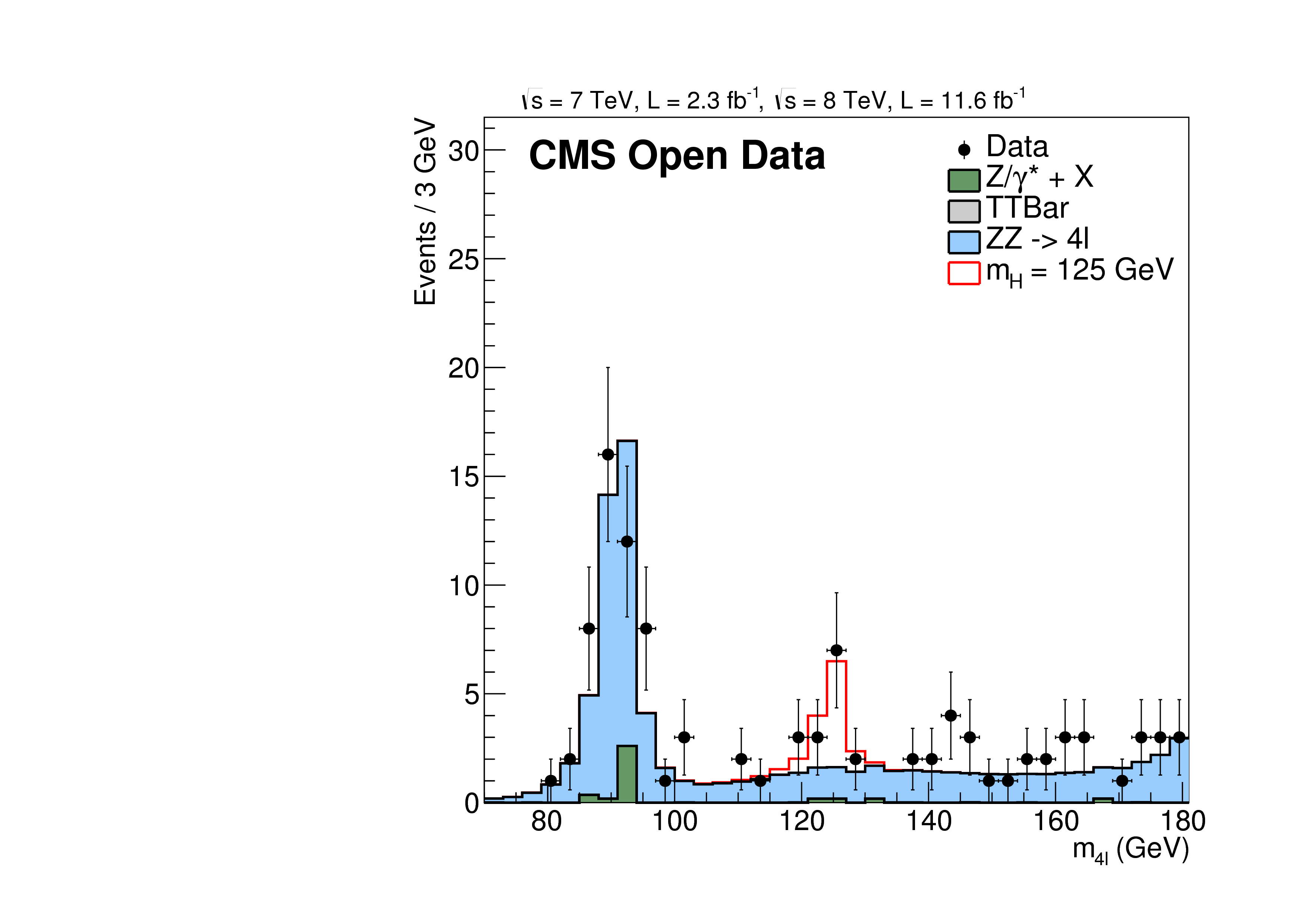
This research level example is a strongly simplified reimplementation of parts of the original CMS Higgs-to-four-lepton analysis published in Phys.Lett. B716 (2012) 30-61, arXiv:1207.7235, https://inspirehep.net/record/1124338?ln=en
The published reference plot which is being approximated in this example is
https://inspirehep.net/record/1124338/files/H4l_mass_v3.png
Other Higgs final states (e.g. Higgs to two photons), which were also part of
the same CMS paper and strongly contributed to the Higgs discovery, are not
covered by this example.
The highest level, of this example addresses users who feel they have at least some minimal understanding of the content of this paper and of the meaning of this reference plot, which can be reached via (separate) educational exercises. The lower levels might also be interesting for educational applications. The example requires a minimal acquaintance with the linux operating system and the Root analysis tool, which can also be obtained from corresponding (separate) tutorials.
The example uses legacy versions of the original CMS data sets in the CMS AOD format, which slightly differ from the ones used for the publication due to improved calibrations. It also uses legacy versions of the corresponding Monte Carlo simulations, which are again close to, but not identical to, the ones in the original publication. These legacy data and MC sets listed below were used in practice, exactly as they are, in many later CMS publications.
Since according to the CMS Open Data policy the fraction of data which are public (and used here) is only 50% of the available LHC Run I samples, the statistical significance is reduced with respect to what can be achieved with the full dataset. However, the original paper Phys.Lett. B716 (2012) 30-61, arXiv:1207.7235, https://inspirehep.net/record/1124338?ln=en was also obtained with only part of the Run I statistics, roughly equivalent to the luminosity of the public set, but with only partial statistical overlap.
The provided analysis code recodes the spirit of the original analysis and recodes many of the original cuts on original data objects, but does not provide the original analysis code itself. Also, for the sake of simplicity, it skips some of the more advanced analysis methods of the original paper. Nevertheless, it provides a qualitative insight about how the original result was obtained. In addition to the documented core results, the resulting Root files also contain many undocumented plots which grew as a side product from setting up this example and earlier examples. The significance of the Higgs "excess" is about 2 standard deviations in this example, while it was 3.2 standard deviations in this channel alone in the original publication. The difference is attributed to the less sophisticated background suppression. In more recent (not yet public) CMS data sets with higher statistics the signal is observed in an analysis with more than 5 standard deviations in this channel alone in the preliminary result CMS-PAS-HIG-16-041 https://inspirehep.net/record/1518828. The most recent results on the search and observation of the Higgs boson in this decay mode are available here: http://cms-results.web.cern.ch/cms-results/public-results/publications/HIG/ZZ.html
The analysis strategy is the following: Get the 4mu and 2mu2e final states from the DoubleMuParked datasets and the 4e final state from the DoubleElectron dataset. This avoids double counting due to trigger overlaps. All MC contributions except top use data-driven normalization: The DY (Z/gamma^*) contribution is scaled to the Z peak. The ZZ contribution is scaled to describe the data in the independent mass range 180-600 GeV. The Higgs contribution is scaled to describe the data in the signal region. The (very small) top contribution remains scaled to the MC generator cross section.
There are four levels of increasing complexity for this example:
- Compare the provided final output plot mass4l_combine.pdf or mass4l_combine.png to the published one, https://inspirehep.net/record/1124338/files/H4l_mass_v3.png keeping in mind the caveats given above
-
Reproduce the final output plot from the predefined histogram files using a ROOT macro (Time: ~few minutes - ~few hours, depending on setup and proficiency) There are two ways to do this tutorial, with either a local software or virtual installation of the ROOT framework. ROOT is a software framework very commonly used in particle physics.
If not already proficient in ROOT, consider doing a brief ROOT introductory tutorial [https://root.cern.ch/introductory-tutorials] in order to understand what the ROOT macro will do .
if a ROOT version on the local computer compatible with ROOT 5.32/00 is running, use the local version. This avoids installation of the CERN VM.
If you do not have ROOT installed, it is also possible to run this part of the tutorial in the CERN Virtual Machine. Follow the instructions in the Prerequisites section of the Level 3 tutorial]in order to install the Virtualbox and CERNVM and run ROOT in the virtual machine [http://opendata.cern.ch/VM/CMS/2011]
-
download the git repository, in this case you get the directory structure automatically.
For those who want to set things up, there also is a complete tutorial on the CMS Open Data portal that walks you through a full setup including all directory structures.
In this tutorial we have done this for you.
git clone git://github.com/cms-opendata-analyses/HiggsExample20112012.git
cd HiggsExample20112012/
ls
What you will see is that there are multiple directories called
Level2,Level3,Level4,rootfiles, etc.For now we will focus on the
Level2tutorial.The
HiggsExample20112012package already includes a download of all the preproduced *.root files given in tobereleased for all relevant samples to therootfilesdirectory, so this saves you the exercise of downloading all of these.
In
HiggsExample20112012/Level2you find the fileM4Lnormdatall.ccthis is a root macro that you will run to obtain the plots that were considered in the Level 1 part of this tutorial. Particularly for starting users, it would be useful to study the code of this macro in detail to understand what it does. Very important is that this macro loads the files present in theHiggsExample20112012/rootfilesdirectory, combines this information into a final plot, that the macro will save.-
on the linux prompt, with ROOT installed, and in the
HiggsExample20112012/Level2directory, typeroot -l M4Lnormdatall.cc-> you will get the output plot on the screen
-
either, on the ROOT canvas (picture) click
file->Quit ROOTor, on the root [] prompt, type the command to end your root session:
.q-> you will exit ROOT and find the output plot in mass4l_combined_user.pdf
-
you can compare this plot with the plots provided in 1.
-
-
Produce a ROOT data input file from original data and MC files for one Higgs signal candidate and for the simulated Higgs signal with reduced statistics (for speed reasons) and reproduce the final output plot containing your own input using a ROOT macro (~few minutes to ~1 hour if Virtual machine is already installed, depending on internet connection and computer performance, up to ~few hours otherwise)
-
if not already done follow instructions in CMS 2011 Virtual Machines: How to install
[http://opendata.web.cern.ch/docs/cms-virtual-machine-2011]- install VirtualBox
- install CERNVM Virtual Machine
-
install the CMSSW software environment
cmsrel CMSSW_5_3_32And then move into the working (
src) directory and setup the computing environmentcd CMSSW_5_3_32/src cmsenvYou now have a working ROOT environment and all CMS code framework at your disposal. Next step is to add analysis code.
-
optional: for better understanding of the code used in the following steps, it is highly recommended to also work through the Test & Validate section of the [http://opendata.web.cern.ch/docs/cms-virtual-machine-2011] instructions.
-
If you have not already done so, download and install the code.
git clone git://github.com/cms-opendata-analyses/HiggsExample20112012.git -
For this example, all active code and macros are present in the
HiggsExample20112012/Level3directories. The analysis code in c++ that you will run is present inHiggsExample20112012/HiggsDemoAnalyzerdirectory, and it will need to be compiled. You will also use the files in theHiggsExample20112012/rootfilesdirectory when making the final plot, similar to the Level2 tutorial.cd HiggsExample20112012/HiggsDemoAnalyzer -
The code in this directory calls analysis code that is very similar to the one used in the
Demo/DemoAnalyzertutorial (which you should be familiar with from the [http://opendata.web.cern.ch/docs/cms-virtual-machine-2011] tutorials). To compile the code you typescram b -
Now you should have a working version of the
HiggsDemoAnalyzeravailable in your environment. You can check this with theedmPluginDumpcommand, or more usefuledmPluginDump | grep HiggsDemoAnalyzer. You should see a printout of the HiggsDemoAnalyzerGit name twice.
-
In your
HiggsExample20112012/Level3directory you should see the filesdemoanalyzer_cfg_level3data.py(data example) anddemoanalyzer_cfg_level3MC.py(Higgs simulation example)# from HiggsExample20112012/HiggsDemoAnalyzer cd ../Level3 ls -
The data conditions when the CMS detector was taking data of high enough quality are stored in files of the json format. You can download the 2012 validation file from [http://opendata.web.cern.ch/record/1002], in the same link there also are details on how the good-data selection is made. In this example the file has already been copied to the repository, it is the file
datasets/Cert_190456-208686_8TeV_22Jan2013ReReco_Collisions12_JSON.txt. -
run the two analysis jobs (one on data, one on MC, the input files are already predefined)
cmsRun demoanalyzer_cfg_level3data.pywill produce output file
DoubleMuParked2012C_10000_Higgs.rootcontaining 1 Higgs candidate from the data.cmsRun demoanalyzer_cfg_level3MC.pywill produce output file
Higgs4L1file.rootcontaining the Higgs signal distributions with reduced statistics -
Analogous to the Level 2 example, you will now use a ROOT macro
M4Lnormdatall_lvl3.ccto analyse the files inrootfiles. However, besides that, you will add your own one extra data point that you have processed, and you will use your own higgs boson signal histogram, which both are loaded from the histograms in thelevel3directory!- it is worthwhile to take a look at the
M4Lnormdatall_lvl3.ccmacro, you can identify where the files are loaded and paths are set.
- it is worthwhile to take a look at the
-
on the linux prompt and in your
HiggsExample20112012/Level3directory, typeroot -l M4Lnormdatall_lvl3.cc-> you will get the output plot on the screen; the magenta Higgs signal histogram will now be the one you produced, and the one data event which you have selected will be shown as a blue triangle
-
to exit ROOT, either, on the ROOT canvas (picture) click
file->Quit ROOTor, on the root [] prompt, type.q-> you will exit ROOT and find the output plot in mass4l_combined_user3.pdf
-
you can compare this plot with the plots provided in the Level 1 tutorial.
-
- Reproduce the full example analysis (up to ~1 month or more on single CPU with fast internet connection, depending on internet connection speed and computer performance)
-
start by running the Level 3 and understand what you have done
-
the Level 4 tutorial has very similar structure as the Level 3 tutorial. The analysis control files are present in the
HiggsExample20112012/Level4and allow to run over full datasets of millions of LHC data and simulation events. -
at this level, instead of running over a single file, you will run over so-called index files which contain lists (
chains) of many files -
the data index files for the datasets listed in List_indexfile.txt to the datasets directory, which you have to download from the CMS data portal http://opendata.cern.ch/record/5500. The configuration files should run out of the box on a dataset and a Monte-Carlo simulation file, in this case ZZ boson production, one of the main backgrounds in the plots, the light-blue one.
-
the 2011 validation (JSON) file is present in the datasets directory (in which you should already have the 2012 one)
-
download all the MC index files for the MC sets listed in List_indexfile.txt to the datasets directory, a dedicated directory for the MC index files is already present with one file in there.
-
edit the relevant demoanalyzer file and insert the index file you want; for data, make sure to use the correct JSON validation file in each case; set an outputfile name of your choice for each smaple which you will recognise. Important:
- modify input file
- modify name output file
- if the input file is data, you need to use the validation (JSON) file appropriate to the run period, so either 2011 or 2012.
-
run the analysis job (cmsRun demoanalyzer_cfg_level4...) sequentially on all the input samples listed in List_indexfile.txt, i.e. produce all root output files yourself.
If you have access to a computer farm with local support for the installation of the CMS software (the Open Data team can only provide support for the single virtual machine mode), you may also run the analysis in parallel on different CPUs, correspondingly speeding up the result.
-
merge all the files from different index files of a dataset by using ROOT tools . For example the
haddcommand allows you to merge root files. If you move all files into a single directory and use the same naming convention as indatafilesit should only be a straightforward modification of the path at the start of the Level 2 macros that would allow you to run. -
You can then repeat the Level 2 part of this exercise, using your own ROOT output files instead of the predefined ones. Or plot whatever properties you want after modifying the macros! Enjoy!
FB would like to thank ATLAS colleagues C. Nellist and A. Elliot for their valuable time and help to test this tutorial.