Brought to you by Lesley Cordero.
- 0.0 Setup
- 1.0 Background
- 2.0 LSTM Networks
- 3.0 gensim and nltk
- 4.0 Convolution Neural Networks
- 5.0 Final Words
This guide was written in Python 3.5.
pip3 install tensorflow
pip3 install gensim
pip3 install nltk
If you haven't already, run the following command into your terminal
sudo python3 -m nltk.downloader all
If you'd like to work in a virtual environment, you can set it up as follows:
pip3 install virtualenv
virtualenv your_env
And then launch it with:
source your_env/bin/activate
To execute the visualizations in matplotlib, do the following:
cd ~/.matplotlib
nano matplotlibrc
And then, write backend: TkAgg in the file. Now you should be set up with your virtual environment!
Cool, now we're ready to start!
Working off of the knowledge we gained from previous workshops, we'll spend this tutorial covering the basics of how Deep Learning and Natural Language Processing fields intersect.
With that said, we'll begin by overviewing some of the fundamental concepts of this intersection.
A vector space search involves converting documents into vectors, where each dimension within the vectors represents a term. VSMs represent embedded words in a continuous vector space where semantically similar words are mapped to nearby points.
Vector Space Model methods depend highly on the Distributional Hypothesis, which states that words that appear in the same contexts share semantic meaning. The different approaches that leverage this principle can be divided into two categories: count-based methods and predictive methods.
To begin implementing a Vector Space Model, first you must get all terms within documents and clean them. A tool you will likely utilize for this process is a stemmer, takes words and reduces them to the unchanging portion. Words which have a common stem often have similar meanings, which is why you'd likely want to utilize a stemmer.
We will also want to remove any stopwords, such as a, am, an, also ,any, and, etc. Stop words have little value in this search so it's better that we just get rid of them.
Just as we've seen before, this is what that code might look like:
from nltk import PorterStemmer
stemmer = PorterStemmer()

def removeStopWords(stopwords, list):
    return([word for word in list if word not in stopwords])


def tokenise(words, string):
    string = self.clean(string)
    words = string.split(" ")
return ([self.stemmer.stem(word,0,len(word)-1) for word in words])Next, we'll map the vector dimensions to keywords using a dictionary.
def getVectorKeywordIndex(documentList):
        """create the keyword associated to the position of the elements within the document vectors"""

        # Maps documents into a single word string
        vocabularyString = " ".join(documentList)

        vocabularyList = self.parser.tokenise(vocabularyString)

        vocabularyList = self.parser.removeStopWords(vocabularyList)
        uniqueVocabularyList = util.removeDuplicates(vocabularyList)

        vectorIndex={}
        offset=0
        # Associate a position with the keywords which maps to the dimension on the vector used to represent this word
        for word in uniqueVocabularyList:
                vectorIndex[word]=offset
                offset+=1
return(vectorIndex) We use the Simple Term Count Model to map the documents
def makeVector(wordString):

        # Initialise vector with 0's
        vector = [0] * len(self.vectorKeywordIndex)
        wordList = self.parser.tokenise(wordString)
        wordList = self.parser.removeStopWords(wordList)
        for word in wordList:
                vector[self.vectorKeywordIndex[word]] += 1; # Use Simple Term Count Model
return(vector)We now have the ability to find related documents. We can test if two documents are in the same concept space by looking at the the cosine of the angle between the document vectors. We use the cosine of the angle as a metric for comparison. If the cosine is 1 then the angle is 0° and hence the vectors are parallel (and the document terms are related). If the cosine is 0 then the angle is 90° and the vectors are perpendicular (and the document terms are not related).
We calculate the cosine between the document vectors in python using scipy.
def cosine(vector1, vector2):
        """related documents j and q are in the concept space by comparing the vectors:
                cosine  = ( V1 * V2 ) / ||V1|| x ||V2|| """
return(float(dot(vector1,vector2) / (norm(vector1) * norm(vector2))))In order to perform a search across keywords we need to map the keywords to the vector space. We create a temporary document which represents the search terms and then we compare it against the document vectors using the same cosine measurement mentioned for relatedness.
def search(searchList, documentVectors):
        """ search for documents that match based on a list of terms """
        queryVector = self.buildQueryVector(searchList)

        ratings = [util.cosine(queryVector, documentVector) for documentVector in documentVectors]
        ratings.sort(reverse=True)
return(ratings)Autoencoders are a type of neural network designed for dimensionality reduction; in other words, representing the same information with fewer numbers. A wide range of autoencoder architectures exist, including Denoising Autoencoders, Variational Autoencoders, or Sequence Autoencoders.
The basic premise is simple — we take a neural network and train it to spit out the same information it’s given. By doing so, we ensure that the activations of each layer must, by definition, be able to represent the entirety of the input data.
If each layer is the same size as the input, this becomes trivial, and the data can simply be copied over from layer to layer to the output. But if we start changing the size of the layers, the network inherently learns a new way to represent the data. If the size of one of the hidden layers is smaller than the input data, it has no choice but to find some way to compress the data.
And that’s exactly what an autoencoder does. The network starts out by “compressing” the data into a lower-dimensional representation, and then converts it back to a reconstruction of the original input. If the network converges properly, it will be a more compressed version of the data that encodes the same information.
It’s often helpful to think about the network as an “encoder” and a “decoder”. The first half of the network, the encoder, takes the input and transforms it into the lower-dimensional representation. The decoder then takes that lower-dimensional representation and converts it back to the original image (or as close to it as it can get). The encoder and decoder are still trained together, but once we have the weights, we can use the two separately — maybe we use the encoder to generate a more meaningful representation of some data we’re feeding into another neural network, or the decoder to let the network generate new data we haven’t shown it before.
Because some of your features may be redundant or correlated, you can end up with wasted processing time and an overfitted model - Autoencoders help us avoid that.
Like an autoencoder, this type of model learns a vector space embedding for some data. For tasks like speech recognition we know that all the information required to successfully perform the task is encoded in the data. However, natural language processing systems traditionally treat words as discrete atomic symbols, and therefore 'cat' may be represented as Id537 and 'dog' as Id143. These encodings are arbitrary, and provide no useful information to the system regarding the relationships that may exist between the individual symbols.
This means that the model can leverage very little of what it has learned about 'cats' when it is processing data about 'dogs' (such that they are both animals, four-legged, pets, etc.). Representing words as unique, discrete IDs furthermore leads to data sparsity, and usually means that we may need more data in order to successfully train statistical models. However, using vector representations can overcome some of these obstacles.
Word2vec is an efficient predictive model for learning word embeddings from raw text. It comes in two models: the Continuous Bag-of-Words model (CBOW) and the Skip-Gram model. Algorithmically, these models are similar, except that CBOW predicts target words (e.g. 'mat') from source context words ('the cat sits on the'), while the skip-gram does the inverse and predicts source context-words from the target words.
The easiest way to think about word2vec is that it figures out how to place words on a graph in such a way that their location is determined by their meaning. In other words, words with similar meanings will be clustered together. More interestingly, though, is that the gaps and distances on the graph have meaning as well. So if you go to where “king” appears, and move the same distance and direction between “man” and “woman”, you end up where “queen” appears. And this is true of all kinds of semantic relationships! You can look at this visualization here.
Put more mathematically, you can think of this relationship as:
[king] - [man] + [woman] ~= [queen]
The input of the skip-gram model is a single word, wn. For example, in the following sentence:
I drove my car to school.
"car" could be the input, or "school".
The output of a skip-gram model is the words in wn's context. Going along with the example from before, the output would be:
{"I","drove","my","to","school"}
This output is defined as {wO,1 , ... , wO,C }, where C is the word window size that you define.
This input is defined as {wO,1 , ... , wO,C }, where C is the word window size that you define. For example, the input could be:
{"I","drove","my","to","school"}
The output of the neural network will be wi. Hence you can think of the task as "predicting the word given its context". Note that the number of words we use depends on your setting for the window size.
I drove my car to school.
"car" could be the output.
Fine-Tuning refers to the technique of initializing a network with parameters from another task (such as an unsupervised training task), and then updating these parameters based on the task at hand. For example, NLP architecture often use pre-trained word embeddings like word2vec, and these word embeddings are then updated during training based for a specific task like Sentiment Analysis.
GloVe is an unsupervised learning algorithm for obtaining vector representations (embeddings) for words. GloVe vectors serve the same purpose as word2vec but have different vector representations due to being trained on co-occurrence statistics.
TensorFlow is an open source library for numerical computation using data flow graphs. We'll be using Tensorflow to implement a CNN for Text Classification later.
Tensors are geometric objects that describe linear relations between geometric vectors, scalars, and other tensors. Elementary examples of such relations include the dot product, the cross product, and linear maps. Geometric vectors, often used in physics and engineering applications, and scalars themselves are also tensors.
In TensorFlow, a Session is the environment you execute graph operations in, which contains the state of Variables and queues. Each session operates on a single graph.
A Graph contains operations and tensors. You can use multiple graphs in your program, but most programs only need a single graph. You can use the same graph in multiple sessions, but not multiple graphs in one session. TensorFlow always creates a default graph, but you may also create a graph manually and set it as the new default. Explicitly creating sessions and graphs ensures that resources are released properly when you no longer need them.
TensorFlow has summaries, which allow you to keep track of and visualize various quantities during training and evaluation. For example, you probably want to keep track of how your loss and accuracy evolve over time. You can also keep track of more complex quantities, such as histograms of layer activations.
Another TensorFlow feature you might use is checkpointing, which is when you save the parameters of your model to restore them later on. Checkpoints can be used to continue training at a later point, or to pick the best parameters setting using early stopping.
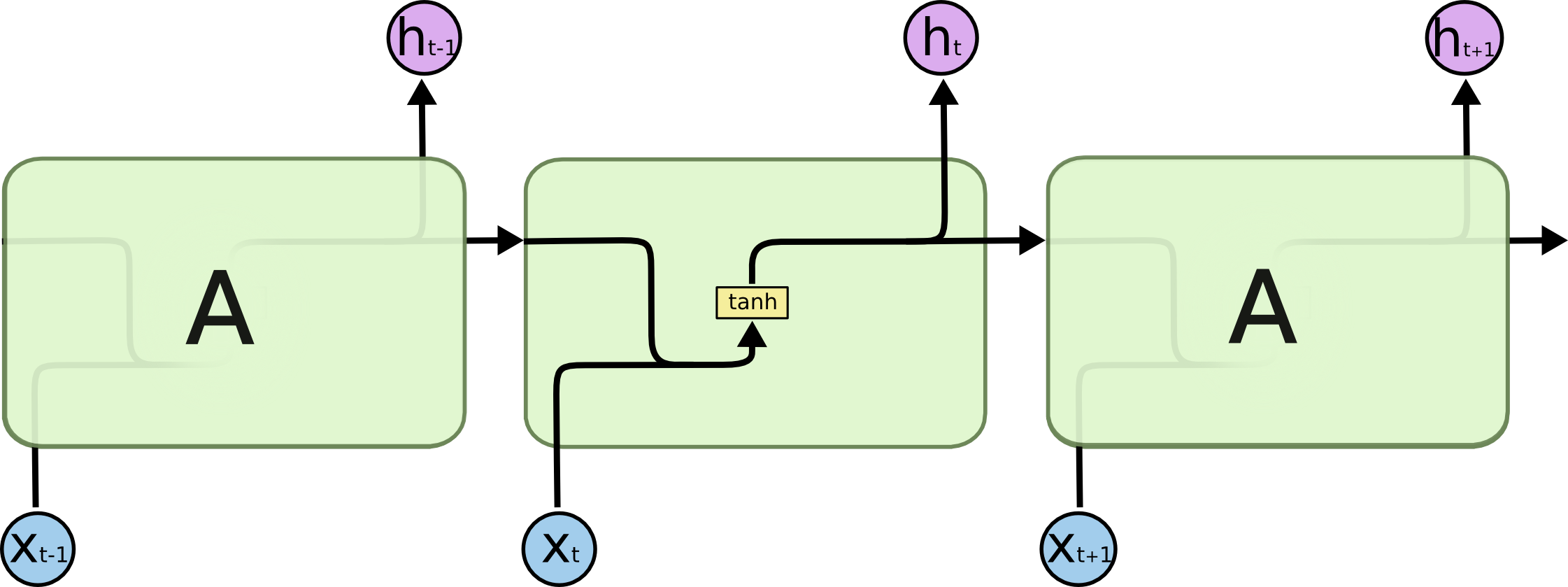
Long Short Term Memory Networks are a special kind of recurrent neural network capable of learning long-term dependencies. LSTMs are explicitly designed to avoid the long-term dependency problem, so remembering information for long periods of time is usually their default behavior.
LSTMs also have the same RNN chain-like structure, but the repeating module has a different structure. Instead of having a single neural network layer, there are four, interacting in a very particular way. You can see that here. Compared to the typical recurrent neural network here, you can see there's a much more complex process happening.
The first step in a LSTM is to decide what information is going to be thrown away from the cell state. This decision is made by a sigmoid layer called the “forget gate layer.” It outputs a number between 00 and 11 for each number in the cell state, where a 1 represents disposal and a 0 means storage.
In the context of natural language processing, the cell state would include the gender of the present subject, so that the correct pronouns can be used in the future.
This next step is deciding what new information is going to be stored in the cell state. First, a sigmoid layer called the “input gate layer” decides which values we’ll update. Secondly, a tanh layer creates a vector of new values that could be added to the cell state.
In our NLP example, we would want to add the gender of the new subject to the cell state, to replace the old one we’re forgetting.
So now we update the old cell state. The previous steps already decided what to do, but we actually do it in this step.
We multiply the old state by new state function, causing it to forget what we've learned earlier. Then we add the updates!
In the case of the language model, this is where we’d actually drop the information about the old subject’s gender and add the new information, which we decided in the previous steps.
Finally, we need to decide what we’re going to output. This output will be based on our cell state, but only once we've filtered it. First, we run a sigmoid layer which decides what parts of the cell state we’re going to output. Then, we put the cell state through tanhtanh (to push the values to be between −1 and 1) and multiply it by the output of the sigmoid gate, so that we only output the parts we need to.
For our NLP example, since it just saw a subject, it might want to output information relevant to a verb, in case that’s what is coming next. For example, it might output whether the subject is singular or plural, so that we know what form a verb should be conjugated into if that’s what follows next.
gensim provides a Python implementation of Word2Vec that works great in conjunction with NLTK corpora. The model takes a list of sentences as input, where each sentence is expected to be a list of words.
Let's begin exploring the capabilities of these two modules and import them as needed:
from gensim.models import Word2Vec
from nltk.corpus import brown, movie_reviews, treebank
Next, we'll load the Word2Vec model on three different NLTK corpora for the sake of comparison.
b = Word2Vec(brown.sents())
mr = Word2Vec(movie_reviews.sents())
t = Word2Vec(treebank.sents())
Here we'll use the word2vec method most_similar to find words associated with a given word. We'll call this method on all three corpora and see how they differ. Note that we’re comparing a wide selection of text from the brown corpus with movie reviews and financial news from the treebank corpus.
print(b.most_similar('money', topn=5))
print(mr.most_similar('money', topn=5))
print(t.most_similar('money', topn=5))
And we get:
[(u'care', 0.9144914150238037), (u'chance', 0.9035866856575012), (u'job', 0.8981726765632629), (u'trouble', 0.8752247095108032), (u'everything', 0.8740494251251221)]

[(u'him', 0.783672571182251), (u'chance', 0.7683249711990356), (u'someone', 0.76824951171875), (u'sleep', 0.7554738521575928), (u'attention', 0.737582802772522)]

[(u'federal', 0.9998856782913208), (u'all', 0.9998772144317627), (u'new', 0.9998764991760254), (u'only', 0.9998745918273926), (u'companies', 0.9998691082000732)]
The results are vastly different! Let's try a different example:
print(b.most_similar('great', topn=5))
print(mr.most_similar('great', topn=5))
print(t.most_similar('great', topn=5))
Again, still pretty different!
[(u'common', 0.8809183835983276), (u'experience', 0.8797307014465332), (u'limited', 0.841762900352478), (u'part', 0.8300108909606934), (u'history', 0.8120908737182617)]

[(u'nice', 0.8149471282958984), (u'decent', 0.8089801073074341), (u'wonderful', 0.8058308362960815), (u'good', 0.7910960912704468), (u'fine', 0.7873961925506592)]

[(u'out', 0.9992268681526184), (u'what', 0.9992024302482605), (u'if', 0.9991806745529175), (u'we', 0.9991364479064941), (u'not', 0.999133825302124)]
And lastly,
print(b.most_similar('company', topn=5))
print(mr.most_similar('company', topn=5))
print(t.most_similar('company', topn=5))
It’s pretty clear from these examples that the semantic similarity of words can vary greatly depending on the textual context.
Convolutional Neural Network (CNNs) are typically thought of in terms of Computer Vision, but they have also had some important breakthroughs in the field of Natural Language Processing. In this section, we'll overview how CNNs can be applied to Natural Language Processing instead.
Instead of image pixels, the input for an NLP model will be sentences or documents represented as a matrix. Each row of the matrix corresponds to one token. These vectors will usually be word embeddings, discussed in section 1 of this workshop, like word2vec or GloVe, but they could also be one-hot vectors that index the word into a vocabulary. For a 10 word sentence using a 100-dimensional embedding we would have a 10×100 matrix as our input. That's what replaces our typical image input.
Previously, our filters would slide over local patches of an image, but in NLP we have these filters slide over full rows of the matrix (remember that each row is a word/token). This means that the “width” of our filters will usually be the same as the width of the input matrix. The height may vary, but sliding windows over 2-5 words at a time is typical.
Putting all of this together, here's what an NLP Convolution Neural Network would look like.
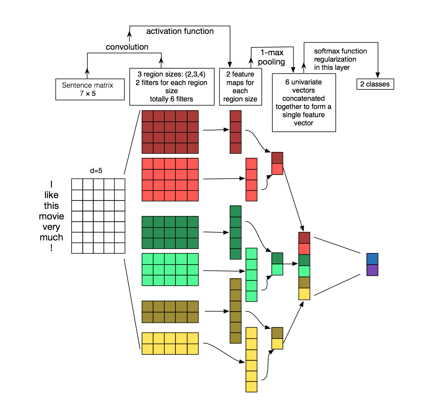
In this portion of the tutorial, we'll be implementing a CNN for text classification, using Tensorflow.
First, begin by importing the needed modules:
import tensorflow as tf
import numpy as np
In this implementation, we'll allow hyperparameter configurations to be customizable so we'll create a TextCNN class, generating the model graph in the init function.
class TextCNN(object):
    def __init__(self, sequence_length, num_classes, vocab_size, embedding_size, filter_sizes, num_filters):
Note the needed arguments to instantiate the class:
- sequence_length: The length of our sentences
- num_classes: Number of classes in the output layer, two in our case.
- vocab_size: The size of our vocabulary.
- embedding_size: The dimensionality of our embeddings.
- filter_sizes: The number of words we want our convolutional filters to cover.
- num_filters: The number of filters per filter size.
We then officially start by defining the input data that we pass to our network:
self.input_x = tf.placeholder(tf.int32, [None, sequence_length], name="input_x")
self.input_y = tf.placeholder(tf.float32, [None, num_classes], name="input_y")
self.dropout_keep_prob = tf.placeholder(tf.float32, name="dropout_keep_prob")
The tf.placeholder creates a placeholder variable that we feed to the network when we execute it at train or test time. The second argument is the shape of the input tensor. None means that the length of that dimension could be anything. In our case, the first dimension is the batch size, and using None allows the network to handle arbitrarily sized batches.
The first layer we define is the embedding layer, which maps vocabulary word indices into low-dimensional vector representations.
with tf.device('/cpu:0'), tf.name_scope("embedding"):
    W = tf.Variable(
        tf.random_uniform([vocab_size, embedding_size], -1.0, 1.0),
        name="W")
    self.embedded_chars = tf.nn.embedding_lookup(W, self.input_x)
self.embedded_chars_expanded = tf.expand_dims(self.embedded_chars, -1)- tf.device("/cpu:0"): This forces an operation to be executed on the CPU. By default TensorFlow will try to put the operation on the GPU if one is available, but the embedding implementation doesn’t currently have GPU support and throws an error if placed on the GPU.
- tf.name_scope: This creates a new Name Scope with the name “embedding”. The scope adds all operations into a top-level node called “embedding” so that you get a nice hierarchy when visualizing your network in TensorBoard.
- W: This is our embedding matrix that we learn during training. We initialize it using a random uniform distribution.
- tf.nn.embedding_lookup: This creates the actual embedding operation. The result of the embedding operation is a 3-dimensional tensor of shape [None, sequence_length, embedding_size].
Now we’re ready to build our convolutional layers followed by max-pooling. Because each convolution produces tensors of different shapes we need to iterate through them, create a layer for each of them, and then merge the results into one big feature vector.
pooled_outputs = []
for i, filter_size in enumerate(filter_sizes):
    with tf.name_scope("conv-maxpool-%s" % filter_size):
        # Convolution Layer
        filter_shape = [filter_size, embedding_size, 1, num_filters]
        W = tf.Variable(tf.truncated_normal(filter_shape, stddev=0.1), name="W")
        b = tf.Variable(tf.constant(0.1, shape=[num_filters]), name="b")
        conv = tf.nn.conv2d(
            self.embedded_chars_expanded,
            W,
            strides=[1, 1, 1, 1],
            padding="VALID",
            name="conv")
        # Apply nonlinearity
        h = tf.nn.relu(tf.nn.bias_add(conv, b), name="relu")
        # Max-pooling over the outputs
        pooled = tf.nn.max_pool(
            h,
            ksize=[1, sequence_length - filter_size + 1, 1, 1],
            strides=[1, 1, 1, 1],
            padding='VALID',
            name="pool")
        pooled_outputs.append(pooled)
Then, we combine all the pooled features:
num_filters_total = num_filters * len(filter_sizes)
self.h_pool = tf.concat(3, pooled_outputs)
self.h_pool_flat = tf.reshape(self.h_pool, [-1, num_filters_total])- W: This is our filter matrix.
- h: This is the result of applying the nonlinearity to the convolution output. Each filter slides over the whole embedding, but varies in how many words it covers.
- "VALID": This padding means that we slide the filter over our sentence without padding the edges, performing a narrow convolution that gives us an output of shape [1, sequence_length - filter_size + 1, 1, 1].
- Performing max-pooling over the output of a specific filter size leaves us with a tensor of shape [batch_size, 1, 1, num_filters]. This is essentially a feature vector, where the last dimension corresponds to our features. Once we have all the pooled output tensors from each filter size we combine them into one long feature vector of shape [batch_size, num_filters_total].
- Using -1 in tf.reshape tells TensorFlow to flatten the dimension when possible.
Dropout is the perhaps most popular method to regularize convolutional neural networks. A dropout layer stochastically disables a fraction of its neurons, which prevents neurons from co-adapting and forces them to learn individually useful features. The fraction of neurons we keep enabled is defined by the dropout_keep_prob input to our network.
with tf.name_scope("dropout"):
    self.h_drop = tf.nn.dropout(self.h_pool_flat, self.dropout_keep_prob)
Using the feature vector from max-pooling (with dropout applied) we can generate predictions by doing a matrix multiplication and picking the class with the highest score. We could also apply a softmax function to convert raw scores into normalized probabilities, but that wouldn’t change our final predictions.
with tf.name_scope("output"):
    W = tf.Variable(tf.truncated_normal([num_filters_total, num_classes], stddev=0.1), name="W")
    b = tf.Variable(tf.constant(0.1, shape=[num_classes]), name="b")
    self.scores = tf.nn.xw_plus_b(self.h_drop, W, b, name="scores")
self.predictions = tf.argmax(self.scores, 1, name="predictions")- tf.nn.xw_plus_b: This is a convenience wrapper to perform the Wx + b matrix multiplication.
We can now define the loss function., which is a measurement of the error our network makes. Remember that our goal is to minimize this function. The standard loss function for categorization problems is the cross-entropy loss, which we implement here:
with tf.name_scope("loss"):
    losses = tf.nn.softmax_cross_entropy_with_logits(self.scores, self.input_y)
    self.loss = tf.reduce_mean(losses)
-tf.nn.softmax_cross_entropy_with_logits: This is the convenience function that calculates the cross-entropy loss for each class, given our scores and the correct input labels. We then take the mean of the losses. We could also use the sum, but that makes it harder to compare the loss across different batch sizes and train/dev data.
We also define an expression for the accuracy, which is a useful quantity to keep track of during training and testing.
with tf.name_scope("accuracy"):
    correct_predictions = tf.equal(self.predictions, tf.argmax(self.input_y, 1))
    self.accuracy = tf.reduce_mean(tf.cast(correct_predictions, "float"), name="accuracy")
And so now we’re done with our network definition!
First, we begin by instantiating our model. By doing so, all of our variables and operations will be placed into our default graphs and sessions.
cnn = TextCNN(
    sequence_length=x_train.shape[1],
    num_classes=2,
    vocab_size=len(vocabulary),
    embedding_size=FLAGS.embedding_dim,
    filter_sizes=map(int, FLAGS.filter_sizes.split(",")),
    num_filters=FLAGS.num_filters)
Next, we define how to optimize our network’s loss function. TensorFlow has several built-in optimizers. We’re using the Adam optimizer.
global_step = tf.Variable(0, name="global_step", trainable=False)
optimizer = tf.train.AdamOptimizer(1e-4)
grads_and_vars = optimizer.compute_gradients(cnn.loss)
train_op = optimizer.apply_gradients(grads_and_vars, global_step=global_step)- train_op: This is a newly created operation that we can run to perform a gradient update on our parameters. Each execution is a training step. TensorFlow automatically figures out which variables are “trainable” and calculates their gradients.
- global_step: By passing this to the optimizer we allow TensorFlow handle the counting of training steps for us. The global step will be automatically incremented by one every time you execute train_op.
Now, before we can train our model we also need to initialize the variables in our graph.
sess.run(tf.initialize_all_variables())Let’s now define a function for a single training step, evaluating the model on a batch of data and updating the model parameters.
def train_step(x_batch, y_batch):

    feed_dict = {
      cnn.input_x: x_batch,
      cnn.input_y: y_batch,
      cnn.dropout_keep_prob: FLAGS.dropout_keep_prob
    }
    _, step, summaries, loss, accuracy = sess.run(
        [train_op, global_step, train_summary_op, cnn.loss, cnn.accuracy],
        feed_dict)
    time_str = datetime.datetime.now().isoformat()
    print("{}: step {}, loss {:g}, acc {:g}".format(time_str, step, loss, accuracy))
train_summary_writer.add_summary(summaries, step)- feed_dict: This contains the data for the placeholder nodes we pass to our network. You must feed values for all placeholder nodes, or TensorFlow will throw an error. -train_op: This actually returns nothing, it just updates the parameters of our network.
Finally, we’re ready to write our training loop. First we initialize the batches:
batches = data_helpers.batch_iter(
    zip(x_train, y_train), FLAGS.batch_size, FLAGS.num_epochs)
Then we iterate over batches of our data, call the train_step function for each batch, and occasionally evaluate and checkpoint our model:
for batch in batches:
    x_batch, y_batch = zip(*batch)
    train_step(x_batch, y_batch)
    current_step = tf.train.global_step(sess, global_step)
    if current_step % FLAGS.evaluate_every == 0:
        print("\nEvaluation:")
        dev_step(x_dev, y_dev, writer=dev_summary_writer)
        print("")
    if current_step % FLAGS.checkpoint_every == 0:
        path = saver.save(sess, checkpoint_prefix, global_step=current_step)
print("Saved model checkpoint to {}\n".format(path))If you want to learn more about Deep Learning & Natural Language Processing, check out our meetups for future content! You can also check out the resources section of this workshop for more!