"Cortical Spike Synchrony as a Measure of Input Familiarity"

Korndörfer, C., Ullner, E., García-Ojalvo, J., & Pipa, G. (2017). Cortical Spike Synchrony as a Measure of Input Familiarity. Neural computation, 29(9), 2491-2510.

tl;dr: In the brain, sometimes a group of cortical cells respond to an input in unison, sometimes each neuron has its own rhythm. Why is that and does it mean anything? Maybe temporal order emerges whenever the input hits a group of well-connected excitatory cells, just because they nudge each other and share a resonant frequency. So then, maybe coinciding responses mean that the same group of cells was often hit by similar patterns in the past, since that's where strong, excitatory connections come from.

https://arxiv.org/abs/1709.03113 (open access)

http://www.mitpressjournals.org/doi/abs/10.1162/neco_a_00987 (paywall)

Source files overview

These sources have three parts:

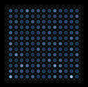
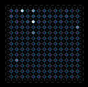
• a numerical simulation of noise-driven FitzHugh-Nagumo and Izhikevich spiking networks written in C.
• a python wrapper for the simulation, offering an epidemic of functions to define & visualize experiments on such networks.
• several python scripts that generate the figure panels shown in the article and some additional plots.

A note on code quality: This is public only because scientific code should be out there, even (or especially) if its creator is not entirely proud of it. It's not a piece of software, just a pile of experiments with a long history of shifting scopes (and old enough to be in python 2, somehow). But fear not! The main pathways are quite well-aired and documented & everything makes colorful plots.

Dependencies

• numpy & matplotlib (http://www.scipy.org/)

• the "networkx" graph library (http://networkx.github.io/)

• the GNU scientific library (http://www.gnu.org/software/gsl/)

• (ffmpeg, but only if you want to export animations. https://www.ffmpeg.org/)

Tested with:

• OSX 10.9 - 10.12, Ubuntu 12.04

• LLVM/clang 8 (via xcode 8.2)

• GNU scientific library 2.2.1

• Python 2.7.11

• Numpy 1.12.0

• matplotlib 2.0.0

• networkx 1.8.1

Installation:

with all dependencies installed,

• compile the simulation using the makefile in libHC/ekkesim (i.e. in that directory, type make izhikevich)
  • in case you have the GSL installed in a non-standard path, you may use make local PREFIX={the path prefix used when configuring & installing the GSL} for convenience. This just passes PREFIX/include and PREFIX/lib to the gcc's -I and -L options, respectively.
• run the example script in an interactive python session: python -i libHC/example.py

Getting started

If your aim is to retrace in detail the computations that lead to each figure, I suggest the following reading order:

• run & read libHC/example.py
• read libHC/hcLab.py, starting with the experiment class. Each such object controls the simulations & measurements for one stimulus condition.
• the interface to the C simulation code is in libHC/hcWrapSim.py. Consider setting a breakpoint at the end of run_sim() in that file to examine the arguments passed to the C simulation & to view its unprocessed output.
• The simulation code is in libHC/ekkesim/src/simulation_izhikevich.c.
• The various figure-generating scripts live in ./figures. they make references to some additional modules e.g. for network generation or for plotting.