Navigating an Agent using a Deep Q-Network

David Rose

2018-12-11

Introduction

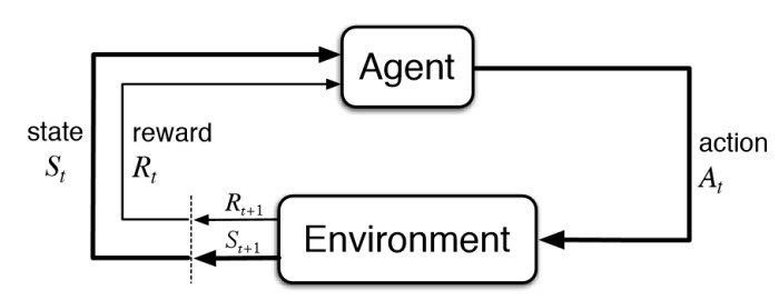
Using a simulated Unity environment, this agent learns a policy of collecting yellow bananas while avoiding blue bananas, using no preset instructions other than the rewards obtained through exploration.

Reinforcement Learning --> Q-Learning --> Deep Q-Learning

Under the umbrella of machine learning, we typically describe 3 foundational perspectives:

1. Unsupervised Learning
2. Supervised Learning
3. Reinforcement Learning

Each of these relate to differing methods of finding patterns in data, but the one we focus on here is reinforcement learning in which we are able to build up an optimal policy of actions using a simulation of positive and/or negative rewards.

The specific model used is referred to as a Deep Q-Network. First proposed by DeepMind in 2015, see paper here in Nature, it attempted to incorporate deep neural networks and traditional Q-Learning into a unified framework that could better generalize between environments, and deal with the larger complexity of continuous state spaces and visual images (relative to the state space of a game such as chess).

The basics of a Q-Network

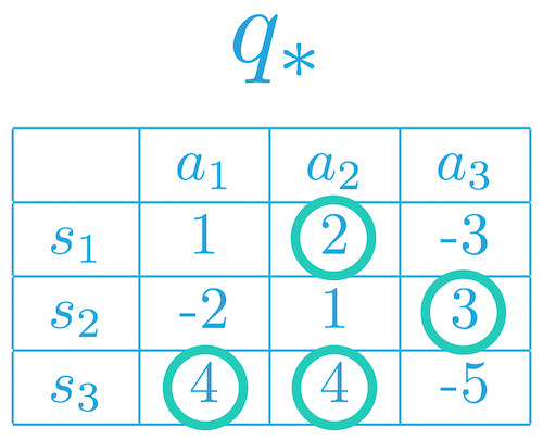
We start with the traditional method of Q-Learning, in which we have a table of possible states and actions Q[S,A], and the expected reward of each combination. When the agent needs to act, it chooses the maximum expected value action for that state, as according to the Q-table. As stated above, this complexity quickly gets out of hand when scaling up environments and we would like to generalize between state/action rewards rather than purely memorizing the past.

As an example: in the table below is a very simple environment in which there are only 3 states and 3 actions. The green circles represent the expected rewards for each combination. While this may be manageable to a human and more complex environments may still be manageable for a computer, eventually the infinitely continuous nature of the real world and the unavoidable issue of exponentially increasing combinations will come with a vengeance.

Enter neural networks

A core idea behind neural networks is pattern fitting, specifically the ability to represent compressed connections from input --> output, which in the case of supervised learning may be image --> cat or audio --> text. In the case of reinforcement learning, we are trying to learn state --> actions/rewards. So given a particular state (for example the relative positions of different bananas compared to my agent) the model will output the expected reward for each action of forward/backward/left/right. It is expected to learn that if a blue banana is in front of me while a yellow is to the left, the agent will turn left and then head forward.

So with these two ideas above we can see how combining them can solve the problems we came across regarding complexity, and the following I think is the most important part to understand:

As opposed to the standard approach of explicitly mapping out a reward to each state/value combination, we can use a neural network as a function approximator.

That is, if there are two locations (states) near each other that continually produce positive rewards, we can generalize that the locations between those two should also produce positive rewards. Now this is a very basic example, but it helps to get the point across.

Below is a diagram of the model that DeepMind used in one of their first attempts at playing through various Atari games. Using the convolutional and fully connected layers, the neural network can progressively learn more-and-more detailed and intricate patterns and connections between the image on the screen, the actions to take, and the expected rewards.

Diagram of Deepmind's DQN for Atari 2600

In the image of above you can see a diagram of how the signal passes from the state spaces to various layers of the neural network, and finally to the different action outputs and their corresponding expected rewards.

In our model we have a more simplified version that uses fully-connected layers, consisting of:

• the state space of 37
• 2 hidden layers (64 nodes each)
• an output of 4 actions

Here is what a diagram of all the layers, nodes, and connections looks like:

(there may be some weird aliasing going on depending on the screen, the original image had to be scaled down a bit)

See this GIST by craffel for the code on making this image.

It looks pretty impressive all laid out like this! But this model is much simpler than most image receiving networks such as the ones for Atari.

Below I have a section of the code used to create the DQN class:

class QNetwork(nn.Module):
    """Actor (Policy) Model"""

    def __init__(self, state_size, action_size, seed, fc1_units=64, fc2_units=64):
        """
        Initialize parameters and build model

        Params
        ======
            state_size (int): Dimension of each state
            action_size (int): Dimension of each action
            seed (int): Random seed
            fc1_units (int): Number of nodes in first hidden layer
            fc2_units (int): Number of nodes in second hidden layer
        """
        super(QNetwork, self).__init__()
        self.seed = torch.manual_seed(seed)
        self.fc1 = nn.Linear(state_size, fc1_units)
        self.fc2 = nn.Linear(fc1_units, fc2_units)
        self.fc3 = nn.Linear(fc2_units, action_size)

    def forward(self, state):
        """Build a network that maps state -> action values"""
        x = F.relu(self.fc1(state))
        x = F.relu(self.fc2(x))
        x = self.fc3(x)  # Action likelihoods
        return x

That is all a high level overview of the basics of this approach, but by itself it would not work very admirably. So below I outline a couple issues and techniques used to overcome them.

Correlated inputs

With this model we are feeding a time-series input of frames that are mostly the same and highly correlated each step which violates the assumption of independent and identically distributed (i.i.d.) inputs. To solve this we implement a couple features:

• Random sampling of past experience
• Fixed target, using two separate networks.

Replay Buffer

Using a store buffer of past experiences, we can then sample from that during training and update the Q-Network with random state/action combinations.

def sample(self):
    """Randomly sample a batch of experiences from memory"""
    experiences = random.sample(self.memory, k=self.batch_size)

    states = torch.from_numpy(np.vstack([e.state for e in experiences if e is not None])).float().to(device)
    actions = torch.from_numpy(np.vstack([e.action for e in experiences if e is not None])).long().to(device)
    rewards = torch.from_numpy(np.vstack([e.reward for e in experiences if e is not None])).float().to(device)
    next_states = torch.from_numpy(np.vstack([e.next_state for e in experiences if e is not None])).float().to(device)
    dones = torch.from_numpy(np.vstack([e.done for e in experiences if e is not None]).astype(np.uint8)).float().to(device)

    return (states, actions, rewards, next_states, dones)

Dual Networks (Target - Local)

When we learn every n_steps, we hold a specific target and compute the loss from the local network states. This keeps us from chasing a moving target and makes for more stable learning.

def learn(self, experiences, gamma):
    """ Update value parameters using given batch of experience tuples

    Params
    ======
        experiences (Tuple[torch.Tensor]): tuple of (s, a, r, s', done) tuples
        gamma (float): discount factor
    """
    states, actions, rewards, next_states, dones = experiences

    # Get max predicted Q values (for next state) from target model
    Q_targets_next = self.qnetwork_target(next_states).detach().max(1)[0].unsqueeze(1)
    # Compute Q targets for current states
    Q_targets = rewards + (gamma * Q_targets_next * (1 - dones))

    # Get expected Q values from local model
    Q_expected = self.qnetwork_local(states).gather(1, actions)

    # Compute loss
    loss = F.mse_loss(Q_expected, Q_targets)
    # Minimize the loss
    self.optimizer.zero_grad()
    loss.backward()
    self.optimizer.step()

    # Update target network
    self.soft_update(self.qnetwork_local, self.qnetwork_target, TAU)

The Environment

In this particular instance, we have a simple environment that consists of 37 dimensions and contains the agent's velocity, along with ray-based perception of objects around agent's forward direction. Given this information, the agent has to learn how to best select actions. Four discrete actions are available, corresponding to:

• 0 - move forward.
• 1 - move backward.
• 2 - turn left.
• 3 - turn right.

Evaluation agent performance in reinforcement learning

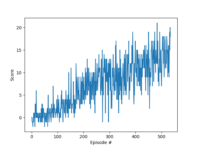
There is no typical standard for identifying when a reinforcement learning agent has solved an environment. It can depend highly on the specific situation and is typically manually identified for each environment. One method is to set a benchmark of reward performance over a certain range of episodes, which for this project is +13 reward average over 100 episodes which was solved in 435 episodes when it was run last.

The image below shows the performance plotted from initialization to final episode.

Improving future performance

The standard DQN is an older baseline algorithm (in the realm of reinforcement learning at least) and there are many improvements and new methods out that have built on these ideas. A lot of work has recently gone into policy-gradient methods that use a deep neural network to specifically map out action probabilities directly from states. These methods are able to harness the powerful computing power of GPUs better, and work well with more complex environments that may utilize raw pixel-level data.

Getting Started

1. Download the environment from one of the links below. You need only select the environment that matches your operating system:

   • Linux: click here
   • Mac OSX: click here
   • Windows (32-bit): click here
   • Windows (64-bit): click here

2. Place the file in the GitHub repository, and unzip (or decompress) the file.

3. Open CMD/Terminal and run 'pip install -r requirements.txt'

4. Run 'python main.py' in your terminal to begin the training process.