Serving Uncertainty

Most Machine Learning (ML) models return a point-estimate of the most likely data label, given an instance of feature data. There are many scenarios, however, where a point-estimate is not enough - where there is a need to understand the model's uncertainty in the prediction. For example, when assessing risk, or more generally, when making decisions to optimise some organisational-level cost (or utility) function. This need is particularly acute when the cost is a non-linear function of the variable you're trying to predict.

For these scenarios, 'traditional' statistical modelling can provide access to the distribution of predicted labels, but these approaches are hard to scale and built upon assumptions that are often invalidated by the data they're trying to model. Alternatively, it is possible to train additional ML models for predicting specific quantiles, through the use of quantile loss functions, but this requires training one new model for every quantile you need to predict, which is inefficient.

Half-way between statistics and ML we have probabilistic programming, rooted in the methods of Bayesian inference. We demonstrates how to train such a predictive model using PyMC3 - a Probabilistic Programming Language (PPL) for Python. We will demonstrate how a single probabilistic program can be used to support requests for point-estimates, arbitrary uncertainty ranges, as well as entire distributions of predicted data labels, for a non-trivial regression task.

We will then demonstrate how to use FastAPI to develop a web API service, that exposes a separate endpoint for each type of prediction request: point, interval and density. Finally, we will walk you through how to deploy the service to Kubernetes, using Bodywork.

All of the files used in this project can be found in the bodywork-pymc3-project repository on GitHub. You can use this repo, together with this guide, to train the model and then deploy the web API to a Kubernetes cluster. Alternatively, you can use this repo as a template for deploying your own machine learning projects. If you're new to Kubernetes, then don't worry - we've got you covered - read on.

A Quick Comment on the Machine Learning Lifecycle

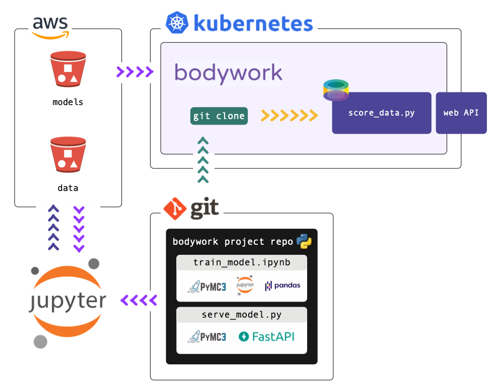
We are going to recommend that the model is trained using the code in the train_model.ipynb notebook. This will persist all ML build artefacts to cloud object storage (AWS S3). We will then use Bodywork to deploy the web API defined in the serve_model.py module, directly from this GitHub repo.

This process should begin as a manual one, and once confidence in this process is establish, re-training can be automated by using Bodywork to deploy a two-stage train-and-serve pipeline that runs on a schedule - e.g., as demonstrated here.

A (very) Quick Introduction to Bayesian Inference

Like statistical data analysis (and ML to some extent), the main aim of Bayesian inference is to infer the unknown parameters in a model of the observed data. For example, to test a hypotheses about the physical processes that lead to the observations. Bayesian inference deviates from traditional statistics - on a practical level - because it explicitly integrates prior knowledge regarding the uncertainty of the model parameters, into the statistical inference process. To this end, Bayesian inference focuses on the posterior distribution,

$$ p(\Theta | X) = \frac{p(X | \Theta) \cdot p(\Theta)}{p(X)} $$

Where,

• $\Theta$ is the vector of unknown model parameters, that we wish to estimate;
• $X$ is the vector of observed data;
• $p(X | \Theta)$ is the likelihood function, that models the probability of observing the data for a fixed choice of parameters; and,
• $p(\Theta)$ is the prior distribution of the model parameters.

The unknown model parameters are not limited to regression coefficients - Deep Neural Networks (DNNs) can be trained using Bayesian inference and PPLs, as an alternative to gradient descent - e.g., see the article by Thomas Wiecki.

If you're interested in learning more about Bayesian data analysis and inference, then an excellent (inspirational) and practical introduction is Statistical Rethinking by Richard McElreath. For a more theoretical treatment try Bayesian Data Analysis by Gelman & co.. If you're curious, read on!

Running the Project Locally

To be able to run everything discussed below, clone the bodywork-pymc3-project repo, create a new virtual environment and install the required packages,

$ git clone https://github.com/bodywork-ml/bodywork-pymc3-project.git
$ cd bodywork-pymc3-project
$ python3.9 -m venv .venv
$ source .venv/bin/activate
$ pip install -r requirements.txt

NOTE - if you're using Apple silicon, then before installing requirements.txt you should run,

brew install hdf5 netcdf
HDF5_DIR=$(brew --prefix hdf5) pip install netcdf4 --no-binary :all:

Getting Started with Kubernetes

If you have never worked with Kubernetes before, then please don't stop here. We have written a Quickstart Guide, that will explain the basic concepts and have you up-and-running with a single-node cluster on your local machine, in under 10 minutes.

Should you want to deploy to a cloud-based cluster in the future, you need only to follow the same steps while pointing to your new cluster. This is one of the key advantages of Kubernetes - you can test locally with confidence that your production deployments will behave in the same way.

Training the Model using PyMC3

A complete Bayesian modelling workflow is covered in-depth and executed within train_model.ipynb. We can summarise the steps in this notebook as follows,

Step 1 - Create an Example Dataset

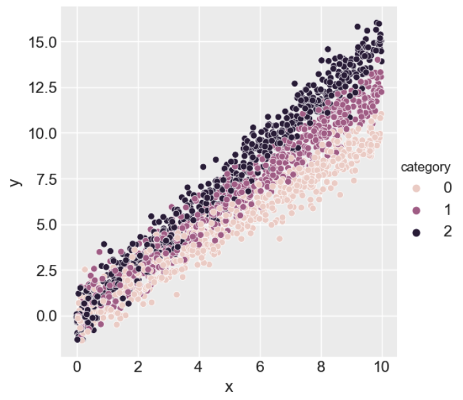
To aid in building intuition for how Bayesian inference and PPLs work, we will simulate a 'toy' regression dataset using random number generation and then estimate the input parameters using the Bayesian inference model defined in Step 2.

For our synthetic dataset, we will assume that the dependent variable (or labelled data), $\tilde{y}$, is a linear function of a single independent variable (or feature), $x$, whose impact on $\tilde{y}$ depends on a categorical variable (or feature), $c$. We define $x$ as a positive real number and $c$ to belong to one of three categories, that occur with equal likelihood. We express this model mathematically, as follows,

$$ \tilde{y} = \beta_{c} \cdot x + \sigma \cdot \tilde{\epsilon} $$

where $\tilde{\epsilon} \sim N(0, 1)$, $\sigma$ is the standard deviation of the random noise in the data and $c \in {0, 1, 2}$ denotes the category. We start by hard-coding our choices for the model parameters.

beta_c0 = 1
beta_c1 = 1.25
beta_c2 = 1.50
sigma = 0.75

We visualise the dataset below.

Step 2 - Define and train a Model

Defining a Bayesian inference model in a PPL like PyMC3, has analogues to defining a DNN model in a tensor computing framework like PyTorch. Perhaps this is not surprising, given that PyMC3 is built upon a tensor computing framework called Aesara. Aesara is a fork of Theano, a precursor of TensorFlow, PyTorch, etc. The model is defined in the following block,

model = pm.Model()

with model:
    # define the variables in the model
    y = pm.Data("y", train["y"])
    x = pm.Data("x", train["x"])
    category = pm.Data("category", train["category"])

    # define the model 
    beta_prior = pm.Normal("beta", mu=0, sd=2, shape=3)
    sigma_prior = pm.HalfNormal("sigma", sd=2, shape=1)
    mu_likelihood = beta_prior[category] * x
    obs_likelihood = pm.Normal("obs", mu=mu_likelihood, sd=sigma_prior, observed=y)

The model encodes our hypothesis about the real-world data-generating process, which in this case is identical to the one used to generate the data. We have made assumptions (or educated guesses) about the prior distribution of all the parameters in the model.

Training the model, means inferring the posterior distribution $p(\Theta | X)$ - the probability of the parameters conditional on the observed data. PPLs use a class of algorithms known as Markov-Chain Monte Carlo (MCMC), to generate samples from the posterior distribution, thereby reconstructing it numerically.

The output of the inference step is basically a dataset - i.e. the collection samples for every parameter in model. You could view MCMC as the analogue of gradient descent for training DNNs, whose aim is to output a set of weights that optimise a loss function, given a model (the network). We execute the inference step with the following block,

with model:
    inference = pm.sample(draws=5000, tune=1000, cores=2, return_inferencedata=True)

Training diagnostics are discussed within the notebook, but it is possible to summarise the inference data with a single visualisation, shown below.

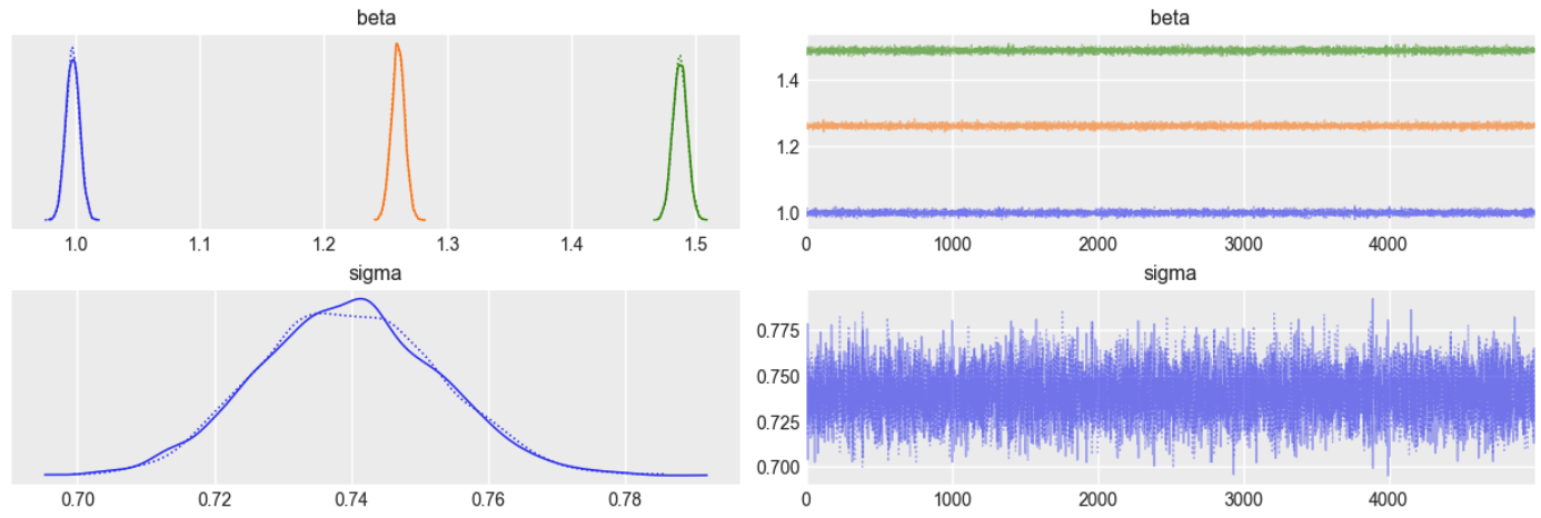
On the left-hand side, the plot shows the distribution of samples for each parameter in the model. We compute the mean of each distribution as:

• beta_0 = 0.996
• beta_1 = 1.248
• beta_2 = 1.510
• sigma = 0.766

Which are very close to the original parameters used to generate the dataset (as you'd hope).

On the right-hand side, the same samples are plotted, but in the sequence in which they were generated by the MCMC algorithm (from which we infer that the simulation is 'stable').

Step 3 - Testing the Model

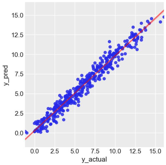
The output from the MCMC algorithm allows us to draw samples of the models' parameters. We choose to draw 100 samples, which enables us to generate 100 possible predictions for every instance of feature data - i.e., we generate a distribution of predicted data labels, for each instance of feature data we want to score.

Most performance metrics for ML models require a point-estimate of the predicted label, not a distribution. We have chosen to compute the mean (expected) label for every set of predicted label samples, so we can compare a single prediction to the actual value and compute the Mean Absolute Percentage Error (MAPE).

with model:
    pm.set_data({
        "y": test["y"],
        "x": test["x"],
        "category": test["category"]
    })
    posterior_pred = pm.sample_posterior_predictive(
        inference.posterior, samples=100
    )

predictions = np.mean(posterior_pred["obs"], axis=0)
mape = mean_absolute_percentage_error(test["y"], predictions)
print(f"mean abs. pct. error = {mape:.2%}")

We visualise the model's performance below.

The model and the inference data are finally uploaded to AWS S3, from where they can be loaded by the web API application, prior to starting the server.

Engineering the Web API using FastAPI

The ultimate aim of this tutorial, is to serve predictions from a probabilistic program, via a web API with multiple endpoints. This is achieved in a Python module we’ve named serve_model.py, parts of which will be reproduced below.

This module loads the trained model that is persisted to cloud object storage when train_model.ipynb is run. Then, it configures FastAPI to start a server with HTTP endpoints at:

• /predict/v1.0.0/point - for returning point-estimates.
• /predict/v1.0.0/interval - for returning highest density intervals.
• /predict/v1.0.0/density - for returning the probability density (in discrete bins).

These endpoints are defined in the following functions (refer to serve_model.py for complete details),

@app.post("/predict/v1.0.0/point", status_code=200)
def predict_point_estimate(request: PointPredictionRequest):
    """Return point-estimate prediction."""
    y_pred_samples = generate_label_samples(
        request.data.x, request.data.category, request.algo_param.n_samples
    )
    y_pred = np.median(y_pred_samples)
    return {"y_pred": y_pred, "algo_param": request.algo_param.n_samples}


@app.post("/predict/v1.0.0/interval", status_code=200)
def predict_interval(request: IntervalPredictionRequest):
    """Return point-estimate prediction."""
    y_pred_samples = generate_label_samples(
        request.data.x, request.data.category, request.algo_param.n_samples
    )
    y_hdi = pm.hdi(y_pred_samples, request.hdi_probability)
    return {
        "y_pred_lower": y_hdi[0],
        "y_pred_upper": y_hdi[1],
        "algo_param": request.algo_param.n_samples,
    }


@app.post("/predict/v1.0.0/density", status_code=200)
def predict_density(request: DensityPredictionRequest):
    """Return density prediction."""
    y_pred_samples = generate_label_samples(
        request.data.x, request.data.category, request.algo_param.n_samples
    )
    y_pred_density, bin_edges = np.histogram(
        y_pred_samples, bins=request.bins, density=True
    )
    bin_mids = 0.5 * (bin_edges[:-1] + bin_edges[1:])
    return {
        "y_pred_bin_mids": bin_mids.tolist(),
        "y_pred_density": y_pred_density.tolist(),
        "algo_param": request.algo_param.n_samples,
    }

Instances of data, serialised as JSON, can be sent to these endpoints as HTTP POST requests. The schema for the JSON data payload are defined by the classes that inherit from pydantic.BaseModel, as reproduced below.

class FeatureDataInstance(BaseModel):
    """Pydantic schema for instances of feature data."""

    x: float
    category: int


class AlgoParam(BaseModel):
    """Pydantic schema for algorithm config."""

    n_samples: int = Field(N_PREDICTION_SAMPLES, gt=0)


class PointPredictionRequest(BaseModel):
    """Pydantic schema for point-estimate requests."""

    data: FeatureDataInstance
    algo_param: AlgoParam = AlgoParam()


class IntervalPredictionRequest(BaseModel):
    """Pydantic schema for interval requests."""

    data: FeatureDataInstance
    hdi_probability: float = Field(0.95, gt=0, lt=1)
    algo_param: AlgoParam = AlgoParam()


class DensityPredictionRequest(BaseModel):
    """Pydantic schema for density requests."""

    data: FeatureDataInstance
    bins: int = Field(5, gt=0)
    algo_param: AlgoParam = AlgoParam()

For more information on defining JSON schemas using Pydantic and FastAPI, see the FastAPI docs.

Testing the web API Locally

You can start the service locally using,

$ python serve_model.py

And test it using,

$ curl http://localhost:8000/predict/v1.0.0/point \
    --request POST \
    --header "Content-Type: application/json" \
    --data '{"data": {"x": 5, "category": 2}}'

{
  "y_pred_lower": 5.997068122059717,
  "y_pred_upper": 8.67981161246493,
  "algo_param": 100
}

And likewise for the other endpoints.

Configuring the Deployment

All configuration for Bodywork deployments must be kept in a YAML file, named bodywork.yaml and stored in the project’s root directory. The bodywork.yaml required to deploy our web API is reproduced below.

version: "1.1"
pipeline:
  name: bodywork-pymc3-project
  docker_image: bodyworkml/bodywork-core:3.0
  DAG: scoring-service
  secrets_group: dev
stages:
  scoring-service:
    executable_module_path: serve_model.py
    requirements:
      - fastapi==0.78.0
      - uvicorn==0.17.6
      - boto3==1.24.13
      - joblib==1.1.0
      - numpy==1.22.1
      - pymc3==3.11.5
    #### you can comment-out this block ####
    secrets:
      AWS_ACCESS_KEY_ID: aws-credentials
      AWS_SECRET_ACCESS_KEY: aws-credentials
      AWS_DEFAULT_REGION: aws-credentials
    ########################################
    cpu_request: 1
    memory_request_mb: 750
    service:
      max_startup_time_seconds: 300
      replicas: 1
      port: 8000
      ingress: true
logging:
  log_level: INFO

Bodywork will interpret this file as follows:

1. Start a Bodywork container on Kubernetes, to run a service stage called scoring-service.
2. Install the Python packages required to run serve_model.py.
3. Mount the AWS credentials contained in the 'aws-credentials' secret, as environment variables accessible to the Python module running in the container. This will automatically configure the AWS client library (boto3) to be able to access your S3 bucket. If you just want to deploy the project from our repo, then you can comment-out the secrets block, as we have the model artefacts stored on publicly accessible S3 buckets that do not require authenticated access. If you want to create a secret for your own credentials, then we will cover this below.
4. Run serve_model.py.
5. Monitor scoring-service and ensure that there is always at least one service replica available, at all times - i.e. it if fails for any reason, then immediately start another one.

Refer to the Bodywork User Guide for a complete discussion of all the options available for deploying machine learning systems using Bodywork.

Deploying the Prediction Service

First of all, if you want inject credentials to access services from your cloud platform, then use (or adapt) the command below. Otherwise, skip this step.

$ bw create secret aws-credentials \
    --secrets-group dev \
    --data AWS_ACCESS_KEY_ID=XX \
    --data AWS_SECRET_ACCESS_KEY=XX \
    --data AWS_DEFAULT_REGION=XX

Next, execute the deployment using,

$ bw create deployment https://github.com/bodywork-ml/bodywork-pymc3-project

Once it has completed, test that the service is responding,

$ curl http://CLUSTER_IP/bodywork-pymc3-project/scoring-service/predict/v1.0.0/point \
    --request POST \
    --header "Content-Type: application/json" \
    --data '{"data": {"x": 5, "category": 2}}'

{
  "y_pred_lower": 5.997068122059717,
  "y_pred_upper": 8.67981161246493,
  "algo_param": 100
}

See our guide to accessing services for information on how to determine CLUSTER_IP.

Congratulations - you have just deployed a probabilistic program ready for production!