GANs are generative models devised by Goodfellow et al. in 2014. In a GAN setup, two differentiable functions, represented by neural networks, are locked in a game. The two players (the generator and the discriminator) have different roles in this framework, as we will se below.
In this repository, I'm trying to generate hand-written digits as below. To do this, I had to learn what is a GAN and how it works.

[Paper] Generative Adversarial Nets : https://arxiv.org/pdf/1406.2661.pdf
[Source] GANs from Scratch 1: A deep introduction. With code in PyTorch and TensorFlow : https://medium.com/ai-society/gans-from-scratch-1-a-deep-introduction-with-code-in-pytorch-and-tensorflow-cb03cdcdba0f
More examples of GANs :

Some of the most relevant GAN pros and cons for the are:
- They currently generate the sharpest images
- They are easy to train (since no statistical inference is required), and only back-propogation is needed to obtain gradients
- GANs are difficult to optimize due to unstable training dynamics.
- No statistical inference can be done with them (except here): GANs belong to the class of direct implicit density models; they model p(x) without explicitly defining the p.d.f.
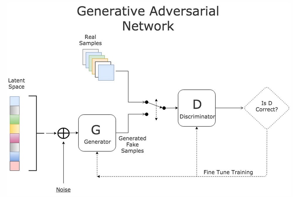
- The first model is called a Generator and it aims to generate new data similar to the expected one. The Generator could be asimilated to a human art forger, which creates fake works of art.
- The second model is named the Discriminator. This model’s goal is to recognize if an input data is ‘real’ — belongs to the original dataset — or if it is ‘fake’ — generated by a forger. In this scenario, a Discriminator is analogous to the police (or an art expert), which tries to detect artworks as truthful or fraud.
The Generator (forger) needs to learn how to create data in such a way that the Discriminator isn’t able to distinguish it as fake anymore. The competition between these two teams is what improves their knowledge, until the Generator succeeds in creating realistic data.
A neural network G(z, θ₁) is used to model the Generator mentioned above. It’s role is mapping input noise variables z to the desired data space x (say images). Conversely, a second neural network D(x, θ₂) models the discriminator and outputs the probability that the data came from the real dataset, in the range (0,1). In both cases, θᵢ represents the weights or parameters that define each neural network.
As a result, the Discriminator is trained to correctly classify the input data as either real or fake. This means it’s weights are updated as to maximize the probability that any real data input x is classified as belonging to the real dataset, while minimizing the probability that any fake image is classified as belonging to the real dataset. In more technical terms, the loss/error function used maximizes the function D(x), and it also minimizes D(G(z)).
Furthermore, the Generator is trained to fool the Discriminator by generating data as realistic as possible, which means that the Generator’s weight’s are optimized to maximize the probability that any fake image is classified as belonging to the real datase. Formally this means that the loss/error function used for this network maximizes D(G(z)).
In practice, the logarithm of the probability (e.g. log D(…)) is used in the loss functions instead of the raw probabilies, since using a log loss heavily penalises classifiers that are confident about an incorrect classification.
After several steps of training, if the Generator and Discriminator have enough capacity (if the networks can approximate the objective functions), they will reach a point at which both cannot improve anymore. At this point, the generator generates realistic synthetic data, and the discriminator is unable to differentiate between the two types of input.
Since both the generator and discriminator are being modeled with neural, networks, agradient-based optimization algorithm can be used to train the GAN. In our coding example we’ll be using stochastic gradient descent, as it has proven to be succesfull in multiple fields.

The fundamental steps to train a GAN can be described as following:
- Sample a noise set and a real-data set, each with size m.
- Train the Discriminator on this data.
- Sample a different noise subset with size m.
- Train the Generator on this data.
- Repeat from Step 1.
TensorBoard : "The computations you'll use TensorFlow for - like training a massive deep neural network - can be complex and confusing. To make it easier to understand, debug, and optimize TensorFlow programs, we've included a suite of visualization tools called TensorBoard. You can use TensorBoard to visualize your TensorFlow graph, plot quantitative metrics about the execution of your graph, and show additional data like images that pass through it."
Leaky ReLU :

Here we’ll use Adam as the optimization algorithm for both neural networks, with a learning rate of 0.0002. The proposed learning rate was obtained after testing with several values, though it isn’t necessarily the optimal value for this task.
The loss function we’ll be using for this task is named Binary Cross Entopy Loss (BCE Loss), and it will be used for this scenario as it resembles the log-loss for both the Generator and Discriminator defined earlier in the post (see Modeling Mathematically a GAN). Specifically we’ll be taking the average of the loss calculated for each minibatch.

In this formula the values y are named targets, v are the inputs, and w are the weights. Since we don’t need the weight at all, it’ll be set to wᵢ=1 for all i.
Discriminator loss :

If we replace vᵢ = D(xᵢ) and yᵢ=1 ∀ i (for all i) in the BCE-Loss definition, we obtain the loss related to the real-images. Conversely if we set vᵢ = D(G(zᵢ)) and yᵢ=0 ∀ i, we obtain the loss related to the fake-images. In the mathematical model of a GAN I described earlier, the gradient of this had to be ascended, but PyTorch and most other Machine Learning frameworks usually minimize functions instead. Since maximizing a function is equivalent to minimizing it’s negative, and the BCE-Loss term has a minus sign, we don’t need to worry about the sign.
Discriminator loss :

Rather than minimizing log(1- D(G(z))), training the Generator to maximize log D(G(z)) will provide much stronger gradients early in training. Both losses may be swapped interchangeably since they result in the same dynamics for the Generator and Discriminator.
Maximizing log D(G(z)) is equivalent to minimizing it’s negative and since the BCE-Loss definition has a minus sign, we don’t need to take care of the sign. Similarly to the Discriminator, if we set vᵢ = D(G(zᵢ)) and yᵢ=1 ∀ i, we obtain the desired loss to be minimized.
DCGAN : Deep Convolutional Generative Adversarial Networks
DCGAN is one of the popular and successful network design for GAN. It mainly composes of convolution layers without max pooling or fully connected layers. It uses convolutional stride and transposed convolution for the downsampling and the upsampling. The figure below is the network design for the generator.

Here is the summary of DCGAN:
- Replace all max pooling with convolutional stride
- Use transposed convolution for upsampling.
- Eliminate fully connected layers.
- Use Batch normalization except the output layer for the generator and the input layer of the discriminator.
- Use ReLU in the generator except for the output which uses tanh.
- Use LeakyReLU in the discriminator.
[Source] http://machinelearninguru.com/computer_vision/basics/convolution/convolution_layer.html


[Source] https://towardsdatascience.com/up-sampling-with-transposed-convolution-9ae4f2df52d0 [Paper] https://arxiv.org/pdf/1603.07285.pdf
When we use neural networks to generate images, it usually involves up-sampling from low resolution to high resolution.
There are various methods to conduct up-sampling operation:
- Nearest neighbor interpolation
- Bi-linear interpolation
- Bi-cubic interpolation
If we want our network to learn how to up-sample optimally, we can use the transposed convolution (also called fractionally-strided convolution or deconvolution). It does not use a predefined interpolation method. It has learnable parameters.
Convolutional operation

One important point of such convolution operation is that the positional connectivity exists between the input values and the output values.
For example, the top left values in the input matrix affect the top left value of the output matrix.
More concretely, the 3x3 kernel is used to connect the 9 values in the input matrix to 1 value in the output matrix. A convolution operation forms a many-to-one relationship. Let’s keep this in mind as we need it later on.
We can express a convolution operation using a matrix.
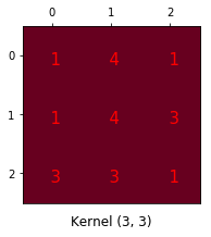
We rearrange the 3x3 kernel into a 4x16 matrix as below:

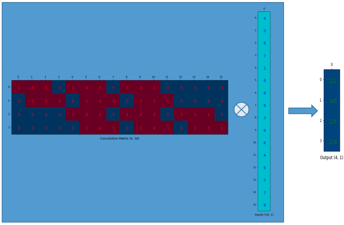
We can matrix-multiply the 4x16 convolution matrix with the 1x16 input matrix (16 dimensional column vector). The output 4x1 matrix can be reshaped into a 2x2 matrix which gives us the same result as before. In short, a convolution matrix is nothing but an rearranged kernel weights, and a convolution operation can be expressed using the convolution matrix.
Going Backward Now, suppose we want to go the other direction. We want to associate 1 value in a matrix to 9 values in another matrix. It’s a one-to-many relationship. This is like going backward of convolution operation, and it is the core idea of transposed convolution.
Going backward of Convolution

We want to go from 4 (2x2) to 16 (4x4). So, we use a 16x4 matrix. But there is one more thing here. We want to maintain the 1 to 9 relationship.
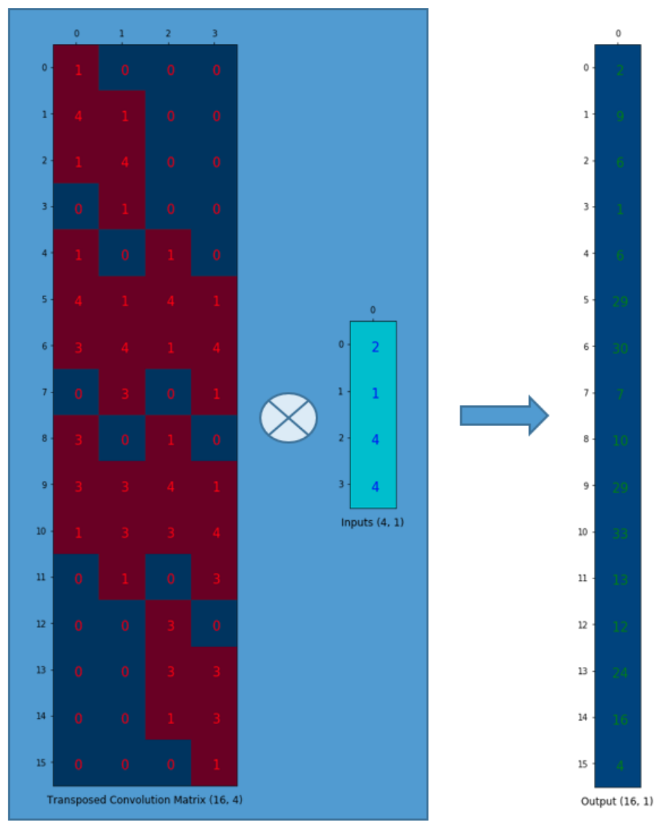
The output can be reshaped into 4x4.
We have just up-sampled a smaller matrix (2x2) into a larger one (4x4). The transposed convolution maintains the 1 to 9 relationship because of the way it lays out the weights.
NB: the actual weight values in the matrix does not have to come from the original convolution matrix. What important is that the weight layout is transposed from that of the convolution matrix.
Moreover, the weights in the transposed convolution are learnable. So we do not need a predefined interpolation method.
One caution: the transposed convolution is the cause of the checkerboard artifacts in generated images. This article recommends an up-sampling operation (i.e., an interpolation method) followed by a convolution operation to reduce such issues. If your main objective is to generate images without such artifacts, it is worth reading the paper to find out more.