SQL_Hypothesis_Testing.ipynb - Notebook inclues data, methodologies and modeling around hypothesis testing
Mod_3_preso.pdf - presentation summarizing findings for a non-technical audience
Additional Files Blog Post: All Data Is NOT Created Normal
*SQL Querying was performed for data extraction for conducting A/B Testing to inform buisiness decisions making for global retailer.
__
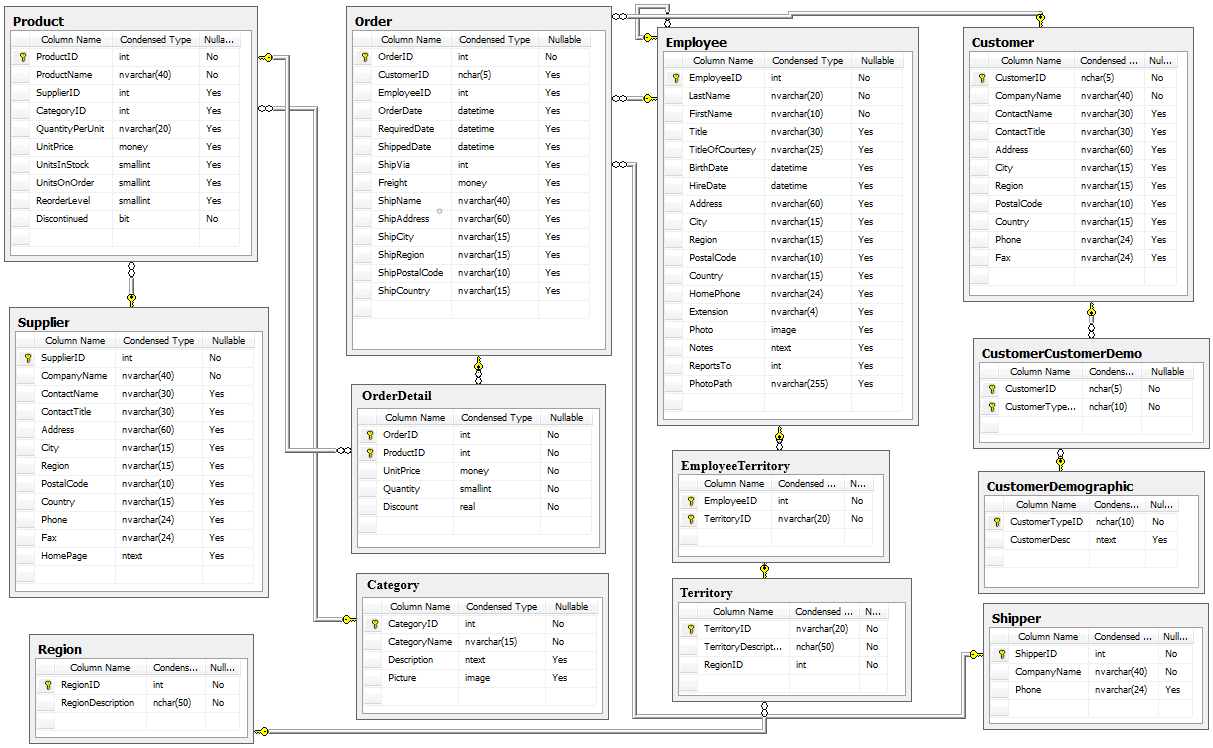
A two year sales history was examined in a series of tables stored in an SQL database. The data provided focused primarly on sales information and did not include cost of goods, so ways were examined to maximize revenues in an effort to improve margins. Several theories were developed and hypothesis were formed around ways to improve revenues.
- Does discount amount have a statistically significant effect on the quantity of a product in an order? If so, at what level(s) of discount?
- Do some categories generate more revenue than others ?? Which ones?
- Do certain sales representatives sell more than others? Who are the top sellers?
- Where are the customers from that spend the most money?
Does discount amount have a statistically significant effect on the quantity of a product in an order? If so, at what level(s) of discount?
-
$H_0$ :There is no statistcally significant effect on the quantity of a product in an order in relation to a discount amount. -
$H_1$ :Discounts have a statistically significant effect on the quantiy of a product in an order. -
$H_1a$ :Certain discount values have a greater effect than others.
To begin, in taking a look at the OrderDetail table, the data required was made available: quantity and discount.
Once imported, the data was grouped by discount level and the means of the quantity sold for each were compared against each other to evaluate if they were statistically significantly different. The results can suggest if the null hypothesis can be rejected with a probability of 5% error in reporting a false negative.
From this dataset of 2155 line items that span 830 orders, it was discovered the average quantity ordered is 24 regardless of discount, the minimum ordered is 0 and max ordered is 130, although the IQR is between 10 and 30. Pricing ranges from $2 - $263 with an average price of $26.21
Discounts were distributed as follows:
0.00    1317
0.05     185
0.10     173
0.15     157
0.20     161
0.25     154
Since we are comparing multiple discounts to inspect it's impact on quantity ordered an AVNOVA or Kruksal test will be run depending on how assumptions are met:
Assumptions for ANOVA Testing were evaluated - Outliers were evaluated using Z-Score Testing and removed. Lavines Testing was conducted on the cleaned dataset and demonstrated that it was not equal variance so Kruksal Wallace testing was conducted. All sample sizes were greater than 15 so the assumption of normality was met.
</style>| group1 | group2 | meandiff | p-adj | lower | upper | reject | |
|---|---|---|---|---|---|---|---|
| 0 | 0.0 | 0.05 | 6.0639 | 0.001 | 2.4368 | 9.6910 | True |
| 2 | 0.0 | 0.15 | 6.9176 | 0.001 | 3.0233 | 10.8119 | True |
| 3 | 0.0 | 0.2 | 5.6293 | 0.001 | 1.7791 | 9.4796 | True |
| 4 | 0.0 | 0.25 | 6.1416 | 0.001 | 2.2016 | 10.0817 | True |
Visual on distributions and potential remaining outliers to get a cleaner view:
#boxen plot
sns.catplot(data=disc_df, x='group', y='data', kind='boxen')
ax.axhline(26.75, color='k')
plt.gca()
plt.show()
This plot may not best suit non-technical audience with the additional information potentially could cause confusion. However, the above boxen plot clearly illustrates distributions as well as remaining potential outliers in the .05, .15, .2 and .25 groups. These outliers were not removed initially with the intention to preserve as much of the initial dataset as possible.
Rejecting the null hypothesis :
- 𝐻0 :There is no statistcally significant effect on the quantity of a product in an order in relation to a discount amount.
Alternative hypothesese:
*  𝐻1 :Discounts have a statistically significant effect on the quantiy of a product in an order.
*  𝐻1𝑎 :Certain discount values have a greater effect than others.(see below for findings)
A 10% discount had no statistical significance on the quantiy purchased.
Discounts extended at 5%, 15%, 20%, and 25% statistically are equal on quantity sold when compared to none offered, with a p-value of .001 meaning there is a .01 percent chance of classifying them as such due to chance. Each have varying effect sizes in compared to orders placed with no discount extended.
| Discount | AvQty | Effect Size | Effect |
|---|---|---|---|
| 5 % | 27 | .1982 | Small |
| 15 % | 27 | .454 | Medium |
| 20 % | 26 | .3751 | Medium |
| 25 % | 27 | .454 | Medium |
Additional notes:
- For discounts 1%,2%,3%,4%, and 6% that were included in the original dataset, the amount of data provided was relatively small to evaluate the impact on the whole. This data was removed from further testing
- With additional outliers removed for each of the discount groups, the revised average qty purchased was 23 overall.
While larger discounts did deomonstrate significant effect on quantity purchased, smaller discounts held a statistically equal effect. To recognize the effect of driving higher quantities purchased and realize larger profit margins, offer the smaller discount(s).
Do some categories generate more revenue than others ?? Which ones?
-
$𝐻0$ : All categories generate equal revenues. -
$𝐻1$ : Certain categories sell at statistically higher rates of revneu than others. -
$𝐻1𝑎$ :
For this round of testing the Product and OrderDetail tables were queried using SQL. These tables includes product information data including: categories, pricing, and discount information to generate revenues.
There are 8 different categories sold in this company that represent 77 products, and the average revenue generated across all categories is $587.00
cats = {}
for cat in catavs['CategoryName'].unique():
    cats[cat] = catavs.groupby('CategoryName').get_group(cat)['Revenue']
In each of the different categories, the products align as such:
There are 10 products in the Dairy Products Category
There are 7 products in the Grains/Cereals Category
There are 5 products in the Produce Category
There are 12 products in the Seafood Category
There are 12 products in the Condiments Category
There are 13 products in the Confections Category
There are 12 products in the Beverages Category
There are 6 products in the Meat/Poultry Category
Outliers were identified and removed via z-score testing, Levene's testing revealed the data was not of equal variance so Kruksal Wallance was conducted. All sample sizes were greater than 15 so the assumption of normality was met.
Kruksal Testing yielded a p-value of 0.0 so we can reject the null hypothesis. However, since there are multiple products compared to each other, further testing is required.
Post-Hoc Testing: This got complicated since we are comparing each product to every other product individually.
The comparison becomes complicated as each product needs to be compared against the other. This was solved by creating a dataframe that compared group 1 (g1) to group 2 (g2) and results of Tukey Testing to determine if there was significant difference were collected. Subsequently Cohen's D was determined for each pair separately to examine individual effect size.
def mult_Cohn_d(tukey_result_df, df_dict):
    '''Using a dataframe from Tukey Test Results and a
    corresponding dictionary, this function loops through
    each variable and returns the adjusted p-value and Cohn_d test'''
    import pandas as pd

    res = [['g1', 'g2','padj', 'd']]
    for i, row in tukey_result_df.iterrows():
        g1 = row['group1']
        g2 = row['group2']
        padj = row['p-adj']
        d = fn.Cohen_d(df_dict[g1], df_dict[g2])

        res.append([g1, g2,padj, d])

    mdc = pd.DataFrame(res[1:], columns=res[0])
    return mdc
The table below illustrates those categories that can reject the null hypothesis that states all categories generate equal revenue. The adjusted probabplity value (padj) reflects probability and the d column illustrates the outcome of the Cohens D test or the effect size.
mult_Cohn_d(tukeyctrues, cats)| g1 | g2 | padj | d | |
|---|---|---|---|---|
| 0 | Beverages | Dairy Products | 0.0010 | -0.351635 |
| 1 | Beverages | Meat/Poultry | 0.0010 | -0.596175 |
| 2 | Beverages | Produce | 0.0010 | -0.520603 |
| 3 | Condiments | Dairy Products | 0.0449 | -0.277491 |
| 4 | Condiments | Meat/Poultry | 0.0010 | -0.517399 |
| 5 | Condiments | Produce | 0.0010 | -0.490099 |
| 6 | Confections | Dairy Products | 0.0010 | -0.340630 |
| 7 | Confections | Meat/Poultry | 0.0010 | -0.600173 |
| 8 | Confections | Produce | 0.0010 | -0.560435 |
| 9 | Dairy Products | Grains/Cereals | 0.0054 | 0.349940 |
| 10 | Dairy Products | Meat/Poultry | 0.0010 | -0.310545 |
| 11 | Dairy Products | Seafood | 0.0010 | 0.525083 |
| 12 | Grains/Cereals | Meat/Poultry | 0.0010 | -0.563832 |
| 13 | Grains/Cereals | Produce | 0.0010 | -0.570886 |
| 14 | Meat/Poultry | Seafood | 0.0010 | 0.754594 |
| 15 | Produce | Seafood | 0.0010 | 0.798069 |
Reject the null hypothesis:
- 𝐻0 : All categories generate equal revenues.
Alternative hypotheis
- 𝐻1 : Certain categories sell at statistically higher rates of revnue than others.
Top three revenue-generating categories: Meat/Poultry, Produce, and Dairy Products.

another look:

Statistically, Meat/Poultry & Produce were statistically equivalent and ranked as top sellers, Dairy & Produce were statiscally equal. (Definition of statistically equal: they returned false value from Tukey test, indicating they had a simliar mean and therefore statiticaly equal with a .05 chance of falsely being classified as such)
| Category | Average Revenue |
|---|---|
| Meat/Poultry | $810.81 |
| Produce | $695.87 |
| Dairy Products | $593.86 |
| Condiments | $455.54 |
| Confections | $426.83 |
| Grains/Cereals | $421.17 |
| Beverages | $399.77 |
| Seafood | $353.61 |
The table(s) above outlines how the various categories compare to each other. If the adjusted p-value in column padj is >.05, they are statistically equal. Conversely of the adjusted p-value 'adjp' is <.05 the two samples are statistically not-equal. This is further examined by the effect size illustrated in column d. d=0.2 be considered a 'small' effect size, 0.5 represents a 'medium' effect size and 0.8 a 'large' effect size.
Notes: Revenue is calculated by subtracting any extended discounts from the salesprice and multiplying that by quantity sold.
- If there are additional products that align with the higher revenue generating categories, that category could be broadened to maximize revenue generating potential.
Example: Meat/Poultry currently has 6 products, this could be expanded. Conversely, the seafood category carries 12 products which could be narrowed. Additional analysis could demonstrate which seafood are the best sellers which would be preserved.
- Knowing what revenue each category generates could potentially influence the ability to appropriately categorize discounts. However, not knowing profit margins - we'd need to take this into consideration.
Do certain sales representatives sell more than others? Who are the top sellers?
__ For this test sql queries were conducted on Product, OrderDetail, Order and Employee Tables These table includes information on:
1) Product information including SalesPrice, Discount and Quantity Sold
2) Sales Representative Information
A dataframe was compiled and a few calculations were made:
#Sales Revenue is calculated by multiplying the adjusted price (accounting for any discounts) times quantity
dfr['SaleRev'] = (dfr['SalesPrice'] * (1-dfr['Discount'])) * dfr['Quantity']
There are 9 employees in this company associated with sales information and the avarage revenue generated by a sales representative is $629.00.
Initial visual inspection indicates roughly uniform distribution in sales revenue, more than half of the sales representatives achieve the average. Additional testing will demonstrate if it is significant.
Since we are comparing multiple discounts to inspect it's impact on quantity ordered an AVNOVA test will be run: Testing revealed again that equal variance did not exist, outliers were removed via z-scores and since sample sizes were greater than 15 these assumptions were met.


Observation: The plot above proved to be misleading since it goes off the mean, it skews the data. Further testing indicates there are no statistical differences between representatives in terms of revenue generated over this time span. The subsequent plot reveals a more accurate depiction of what testing demonstrates.
With some outliers removed, the adjusted average revenue across all sales representatives: $494.72

Both parametric and non parametric tests were conducted, despite indications for non-parametric tests as the dataset(s) did not meet the assupmtion of equal variance. A visual inspection after outlier removal suggested there could be significant variance in the mean and the parametric was run for comparison. The parametric test indicated that the null hypothesis could be rejected. However, post-hoc testing validated the efficacy of the non-parametric test to accept the null hypothesis, with the smallest probability that the outcome was due to chance was well over the accepted rate of .05.
If there is no statistical difference, and effect size is small at best, best practices can still be shared by those who have a higher average revenue, examples 2,3 and 9 still have higher than average sales.
Perhaps a little healthy, insentivised competition might spur increased revenues if not by one, by many. Also, building on knowledge of smaller discounts yielding larger quantities, sales team could increase revenue by being conservative with discount rates.
Where are the customers from that spend the most money?
An SQL query was executed on the OrderDetail and Order tables. These table includes information on:
1) Sales total information
2) Regions where orders shipped to indicating the location of customers
The amount spent takes into account any discounts that were applied:
dfreg['Amount_Spent'] = ((dfreg['UnitPrice'])*(1 - dfreg['Discount']))*dfreg['Quantity'] There are 9 regions, they are Western Europe, South America, Central America, North America, Northern Europe, Scandinavia, Southern Europe, British Isles, and Eastern Europe'.
The average total spend is $587.37
The distribution indicates there may be outliers.

There are 9 regions in reflected in this dataset
The avarage of total spent is $587.37.
Since we are comparing multiple regions to inspect it's impact on quantity ordered an AVNOVA test will be run: Assumptions for ANOVA Testing were examined. Testing revealed again that equal variance did not exist, outliers were removed via z-scores and since sample sizes were greater than 15 these assumptions were met. It should be noted that one region was only slightly over the minimum sample size (n>15) and contained 16 samples.
Kruskal Wallace testing was conducted once again since the data set was not of equal variance and revealed that we could reject the null hypothesis indicating that some regions generated significantly more revenue than others.
** Noting that the sample size of Eastern Europe is relatively small and the confidence interval is much greater to accomodate for it, possibly skewing the results.
The average spend for this dataset accross all regions was $500.
Regional averages were found to be what is reported in the table below:
| Region | Average Revenue |
|---|---|
| Western Europe | $586.93 |
| North America | $570.33 |
| Northern Europe | $510.45 |
| British Isles | $462.33 |
| South America | $424.14 |
| Scandinavia | $325.18 |
| Southern Europe | $289.35 |
| Central America | $276.47 |
| Eastern Europe | `$220.75 |
For each group, the assumption for equal variance was not met and a Kruksal test was conducted. The p value for the nonparametric kruskal test was singificant, which can reject the null hypothesis that all regions spend the same amounts with a 5% degree of error that this is due to chance.

Orders shipped to Western Europe, and North America and Northern Europe generated the highest amount of revenue, statistically these regions are equal:
| Region 1 | Region 2 | MeanDiff | Adj P | Reject Null |
|---|---|---|---|---|
| North America | Northern Europe | -59.8786 | 0.9000 | False |
| North America | Western Europe | 16.5978 | 0.9000 | False |
| Northern Europe | Western Europe | 76.4764 | 0.7992 | False |
For bottom performers that had enough data:
| Region 1 | Region 2 | Adj P |
|---|---|---|
| South America | Southern Europe | 0.2306 |
** Noting that the sample size of Eastern Europe is relatively small and the confidence interval is much greater to accomodate for it, possibly skewing the results.
tukeyr.plot_simultaneous();
Explore best practices from regions that are top performers.
Market analysis for regions that need to be developed.
Leverage knowledge gained regarding categories and discounts.
Since the data provided did not include purchase prices of merchandise, ways were examined to maximize revenues. The datasets were all multi group comparisons and none of the groups met all the assupmtions for parametric testing. All groups called for Kruskal-Wallis and post-hoc testing detailed in this notebook.
It was discovered through hypothesis testing and data analysis, various ways to achieve this through:
* Minimizing discounts
* Broadening revenue generating categories
* Explore best practices from top performing regions: North America, Northern Europe, and Western Europe
* Conduct market analysis on regions that need to be developed: South America, Southern Europe as well as Eastern Europe
In addition, future analysis and testing could provide insight to:
* Develop Regional Markets
* Develop Sales Staff