- Getting started
- How to use
roast - How to use
roast_target - More notes on the
capInfo.xlsfile - Outputs of ROAST software
- Review of simulation data
- How to ask questions
- Acknowledgements
- Notes
- License
After you download the zip file, unzip it, launch your Matlab, make sure you are under the root directory of ROAST (i.e., you can see example/, lib/, and all other files), and then enter:
roast
This will demo a modeling process on the MNI152 head. Specifically, it will use the T1 image of the 6th gen MNI-152 head to build a TES model with anode on Fp1 (1 mA) and cathode on P4 (-1 mA).
There are 3 main functions that you can call: roast(), roast_target() and reviewRes(), which will be covered in Section 2, Section 3, and Section 6, respectively.
roast(subj,recipe,varargin)
subj: file name (can be either relative or absolute path) of the MRI of
the subject that you want to run simulation on. The MRI can be either T1
or T2. If you have both T1 and T2, then put T2 file in the option 'T2'
(see below options for details). If you do not have any MRI but just want
to run ROAST for a general result, you can use the default subject the
MNI152 averaged head (see Example 1) or the New York head (see Example 2).
recipe: how you want to ROAST the subject you specified above. Default
recipe is anode on Fp1 (1 mA) and cathode on P4 (-1 mA). You can specify
any recipe you want in the format of electrodeName-injectedCurrent pair
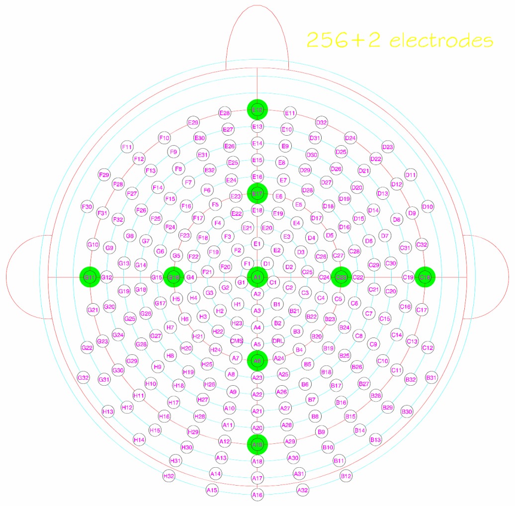
(see Example 3). You can pick any electrode from the 10/20, 10/10, 10/05, BioSemi-256, or EGI HCGSN-256 EEG system (see the Microsoft Excel file capInfo.xls under the root directory of ROAST). The unit of the injected current is in milliampere (mA). Make sure
they sum up to 0. You can also place electrodes at customized locations
on the scalp. See Example 5 for details. You can also use a special recipe called "leadField", so that ROAST will automatically generate all the data that will allow you to call roast_target() later to perform targeted TES. See Example 24 and How to use roast_target.
varargin: Options for ROAST can be entered as Name-Value pairs in the 3rd argument
(available from ROAST v2.0). The syntax follows the Matlab convention (see plot() for example).
If you do not want to read the detailed info on the options below, you can go to Example 23 for quick reference.
'capType' -- the EEG system that you want to pick any electrode from.
'1020' | '1010' (default) | '1005' | 'BioSemi' | 'EGI'
You can also use customized electrode locations you defined. Just provide
the text file that contains the electrode coordinates. See below Example 5 for details.
'elecType' -- the shape of electrode.
'disc' (default) | 'pad' | 'ring'
Note you can specify different shapes to different electrodes, i.e., you
can place different types of electrodes at the same time. See below
Example 6 for details.
'elecSize' -- the size of electrode.
All sizes are in the unit of millimeter (mm). For disc electrodes, sizes
follow the format of [radius height], and default size is [6mm 2mm];
for pad electrodes, sizes follow the format of [length width height], and
default size is [50mm 30mm 3mm]; for ring electrodes, sizes follow the
format of [innerRadius outterRadius height], and default size is [4mm 6mm 2mm].
If you're placing only one type of electrode (e.g., either disc, or pad,
or ring), you can use a one-row vector to customize the size, see Example
7; if you want to control the size for each electrode separately
(provided you're placing only one type of electrode), you need to specify
the size for each electrode correspondingly in a N-row matrix, where N is
the number of electrodes to be placed, see Example 8; if you're placing
more than one type of electrodes and also want to customize the sizes,
you need to put the size of each electrode in a 1-by-N cell (put [] for
any electrode that you want to use the default size), where N is the number
of electrodes to be placed, see Example 9.
'elecOri' -- the orientation of pad electrode (ONLY applies to pad electrodes).
'lr' (default) | 'ap' | 'si' | direction vector of the long axis
For pad electrodes, you can define their orientation by giving the
direction of the long axis. You can simply use the three pre-defined keywords:
'lr'--long axis going left (l) and right (r);'ap'--long axis pointing front (anterior) and back (posterior);'si'--long axis going up (superior) and down (inferior).
For other orientations you can also specify the direction precisely by giving the direction vector of the long axis.
If you're placing pad electrodes only, use the pre-defined keywords
(Example 10) or the direction vector of the long axis (Example 11) to
customize the orientations; if you want to control the
orientation for each pad electrode separately, you need to specify
the orientation for each pad correspondingly using the pre-defined
keywords in a 1-by-N cell (Example 12) or the direction vectors of the
long axis in a N-by-3 matrix (Example 13), where N is the number of pad
electrodes to be placed; if you're placing more than one type of electrodes
and also want to customize the pad orientations, you need to put the
orientations into a N-by-3 matrix (Example 14; or just a 1-by-3 vector or a
single pre-defined keyword if same orientation for all the pads) where N
is the number of pad electrodes, or into a 1-by-N cell (Example 15), where N
is the number of all electrodes to be placed (put [] for non-pad electrodes).
'T2' -- use a T2-weighted MRI to help segmentation.
[] (default) | file path to the T2 MRI
If you have a T2 MRI aside of T1, you can put the T2 file in this option,
see Example 16, note you should put the T1 and T2 files in the same
directory.
If you ONLY have a T2 MRI, put the T2 file in the first argument 'subj'
when you call roast, just like what you would do when you only have a T1.
'meshOptions' -- advanced options of ROAST, for controlling mesh parameters
(see Example 17).
5 sub-options are available:
meshOpt.radbound: maximal surface element size, default 5;meshOpt.angbound: mimimal angle of a surface triangle, default 30;meshOpt.distbound: maximal distance between the center of the surface bounding circle and center of the element bounding sphere, default 0.3;meshOpt.reratio: maximal radius-edge ratio, default 3;meshOpt.maxvol: target maximal tetrahedral element volume, default 10.
See iso2mesh documentation for more details on these options.
'simulationTag' -- a unique tag that identifies each simulation.
dateTime string (default) | user-provided string
This tag is used by ROAST for managing simulation data. ROAST can
identify if a certain simulation has been already run. If yes, it will
just load the results to save time. You can leave this option empty so
that ROAST will just use the date and time as the unique tag for the
simulation. Or you can provide your preferred tag for a specific
simulation (Example 18), then you can find it more easily later. Also all the
simulation history with options info for each simulation are saved in the
log file (named as "subjName_roastLog"), parsed by the simulation tags.
'resampling' -- re-sample the input MRI to 1mm isotropic resolution.
'on' | 'off' (default)
Sometimes the input MRI has a resolution of not being 1 mm, e.g., 0.6 mm.
While higher resolution can give more accurate models, the computation
will be more expensive and thus slower. If you want a faster simulation,
you can ask ROAST to resample the MRI into 1 mm isotropic resolution by
turning on this option (Example 19). Also it is recommended to turn on
this option if your input MRI has anisotropic resolution (e.g., 1 mm by
1.2 mm by 1.2 mm), as the electrode size will not be exact if the model
is built from an MRI with anisotropic resolution. From ROAST v3.0, the data generated by ROAST can be loaded into the Soterix software HD-Explore and HD-Targets, if the input MRI has 1 mm resolution. Users can turn on 'resampling' option for non-1 mm resolution MRI if they want to load the results (only the lead field) in Soterix software later for better visualization. See Example 25.
'zeroPadding' -- extend the input MRI by some amount, to avoid
complications when electrodes are placed by the image boundaries. Default
is not padding any slices to the MRI. You can ask ROAST to pad N empty
slices in all the six directions of the input MRI (left, right, front,
back, up and down), where N is a positive integer. This is very useful
when placing big electrodes on the locations close to image boundaries
(Example 20). This is also useful for MRIs that are cut off at the nose.
If you specify a zeropadding of, say, 60 slices, ROAST can automatically get the segmentation
of the lower part of the head, see (Example 20).
'conductivities' -- advanced options of ROAST, the values are stored as a
structure, with the following field names:
white(default 0.126 S/m);gray(default 0.276 S/m);csf(default 1.65 S/m);bone(default 0.01 S/m);skin(default 0.465 S/m);air(default 2.5e-14 S/m);gel(default 0.3 S/m);electrode(default 5.9e7 S/m).
You can use this option to customize the electrical conductivity for each tissue, each electrode, as well as the conducting medium under each electrode. You can even assign different conductivity values to different electrodes and their conducting media (e.g.,'gel'). See Example 21 and Example 22 for details.
roast
Default call of ROAST, will demo a modeling process on the MNI152 head. Specifically, this will use the MRI of the MNI152 head to build a model of transcranial electric stimulation (TES) with anode on Fp1 (1 mA) and cathode on P4 (-1 mA). Electrodes are modeled by default as small disc electrodes. See options below for details.
roast('nyhead')
ROAST New York head. Again this will run a simulation with anode on Fp1 (1 mA) and cathode on P4 (-1 mA), but on the 0.5-mm resolution New York head. A decent machine of 50GB memory and above is recommended for running New York head. Again electrodes are modeled by default as small disc electrodes. See options below for details.
roast('example/subject1.nii',{'F1',0.3,'P2',0.7,'C5',-0.6,'O2',-0.4})
Build the TES model on any subject with your own "recipe". Here we inject
0.3 mA at electrode F1, 0.7 mA at P2, and we ask 0.6 mA coming out of C5,
and 0.4 mA flowing out of O2. You can define any stimulation montage you want
in the 2nd argument, with electrodeName-injectedCurrent pair. Electrodes are
modeled by default as small disc electrodes. You can pick any electrode
from the 10/20, 10/10, 10/05, BioSemi-256, or EGI HCGSN-256 EEG system. You can find all
the info on electrodes (names, locations, coordinates) in the Microsoft
Excel file capInfo.xls under the root directory of ROAST. Note the unit of
the injected current is milliampere (mA). Make sure they sum up to 0.
roast('example/subject1.nii',{'G12',1,'J7',-1},'captype','biosemi')
Run simulation on subject1 with anode on G12 (1 mA) and cathode on J7 (-1
mA) from the extended BioSemi-256 system (see capInfo.xls under the root
directory of ROAST).
roast('example/subject1.nii',{'E12',0.25,'E7',-0.25,'Nk1',0.5,'Nk3',-0.5,'custom1',0.25,'custom3',-0.25},'captype','egi')
Run simulation on subject1 with recipe that includes: EGI electrodes
E12 and E7; neck electrodes Nk1 and Nk3 (see capInfo.xls); and
user-provided electrodes custom1 and custom3. You can use a free program
called MRIcro to load
the MRI first (note do NOT use MRIcron for this as MRIcron will not give you
the true voxel coordinates) and click the locations on the scalp surface where you want
to place the electrodes, record the voxel coordinates returned by MRIcro
into a text file, and save the text file to the MRI data directory with name
"subjName_customLocations" (e.g., here for subject1 it's saved as
"subject1_customLocations"). ROAST will load the text file and place the
electrodes you specified. You need to name each customized electrode in
the text file starting with "custom" (e.g., for this example they're
named as custom1, custom2, etc. You can of course do
"custom_MyPreferredElectrodeName"). Note that you need to use the MRI that enters ROAST to click for the customized electrode locations (here in this example you need to load 'example/subject1.nii'), even if the MRI is not in RAS orientation, or you turn on the 'resampling' or use 'zeroPadding' option. Just record whatever you get from the original MRI that you used for running ROAST, and ROAST will take care of all the transforms of MRI data (re-orientation into RAS, resampling or zero-padding).
roast([],{'Fp1',1,'FC4',1,'POz',-2},'electype',{'disc','pad','ring'})
Run simulation on the MNI152 averaged head with the specified recipe. A disc electrode will be placed at location Fp1, a pad electrode will be placed at FC4, and a ring electrode will be placed at POz. The sizes and orientations will be set as default.
roast('nyhead',[],'electype','ring','elecsize',[7 10 3])
Run simulation on the New York head with default recipe. Ring electrodes will be placed at Fp1 and P4. The size of each ring is 7mm inner radius, 10mm outter radius and 3mm height.
roast('nyhead',{'Fp1',1,'FC4',1,'POz',-2},'electype','ring','elecsize',[7 10 3;6 8 3;4 6 2])
Run simulation on the New York head with the specified recipe. Ring electrode
placed at Fp1 will have size [7mm 10mm 3mm]; ring at FC4 will have size
[6mm 8mm 3mm]; and ring at POz will have size [4mm 6mm 2mm].
roast([],{'Fp1',1,'FC4',1,'POz',-2},'electype',{'disc','pad','ring'},'elecsize',{[8 2],[45 25 4],[5 8 2]})
Run simulation on the MNI152 averaged head with the specified recipe. A disc
electrode will be placed at location Fp1 with size [8mm 2mm], a pad electrode
will be placed at FC4 with size [45mm 25mm 4mm], and a ring electrode will be
placed at POz with size [5mm 8mm 2mm].
roast([],[],'electype','pad','elecori','ap')
Run simulation on the MNI152 averaged head with default recipe. Pad
electrodes will be placed at Fp1 and P4, with default size of [50mm 30mm 3mm] and the long axis will be oriented in the direction of front to back.
roast([],[],'electype','pad','elecori',[0.71 0.71 0])
Run simulation on the MNI152 averaged head with default recipe. Pad
electrodes will be placed at Fp1 and P4, with default size of [50mm 30mm 3mm] and the long axis will be oriented in the direction specified by the
vector [0.71 0.71 0].
roast('example/subject1.nii',{'Fp1',1,'FC4',1,'POz',-2},'electype','pad','elecori',{'ap','lr','si'})
Run simulation on subject1 with specified recipe. Pad electrodes will be
placed at Fp1, FC4 and POz, with default size of [50mm 30mm 3mm]. The long
axis will be oriented in the direction of front to back for the 1st pad,
left to right for the 2nd pad, and up to down for the 3rd pad.
roast('example/subject1.nii',{'Fp1',1,'FC4',1,'POz',-2},'electype','pad','elecori',[0.71 0.71 0;-0.71 0.71 0;0 0.71 0.71])
Run simulation on subject1 with specified recipe. Pad electrodes will be
placed at Fp1, FC4 and POz, with default size of [50mm 30mm 3mm]. The long
axis will be oriented in the direction of [0.71 0.71 0] for the 1st pad,
[-0.71 0.71 0] for the 2nd pad, and [0 0.71 0.71] for the 3rd pad.
roast([],{'Fp1',1,'FC4',1,'POz',-2},'electype',{'pad','disc','pad'},'elecori',[0.71 0.71 0;0 0.71 0.71])
Run simulation on the MNI152 averaged head with specified recipe. A disc
electrode will be placed at FC4. Two pad electrodes will be placed at Fp1
and POz, with long axis oriented in the direction of [0.71 0.71 0] and
[0 0.71 0.71], respectively.
roast([],{'Fp1',1,'FC4',1,'POz',-2},'electype',{'pad','disc','pad'},'elecori',{'ap',[],[0 0.71 0.71]})
Run simulation on the MNI152 averaged head with specified recipe. A disc
electrode will be placed at FC4. Two pad electrodes will be placed at Fp1
and POz, with long axis oriented in the direction of front-back and [0 0.71 0.71], respectively.
roast('example/subject1.nii',[],'T2','example/subject1_T2.nii')
Run simulation on subject1 with default recipe. The T2 image will be used for segmentation as well.
roast([],[],'meshoptions',struct('radbound',4,'maxvol',8))
Run simulation on the MNI152 averaged head with default recipe. Two of the mesh options are customized.
roast([],[],'simulationTag','roastDemo')
Give the default run of ROAST a tag as 'roastDemo'.
roast('example/subject1.nii',[],'resampling','on')
Run simulaiton on subject1 with default recipe, but resample the MRI of subject1 to 1mm isotropic resolution first (the original MRI of subject1 has resolution of 1mm by 0.99mm by 0.99mm).
roast([],{'Exx19',1,'C4',-1},'zeropadding',60,'simulationTag','paddingExample')
Run simulation on the MNI152 averaged head, but add 60 empty slices on each of the six directions to the MRI first, to allow placement of electrode Exx19, which is outside of the MRI (i.e., several centimeters below the most bottom slice of the MRI). This zeropadding also will generate the segmentation of the lower part of the head, thanks to the extended TPM coming along with ROAST. You can visually check this by
reviewRes([],'paddingExample','all')
If you run this without zero-padding first, you'll get strange results.
Note it is always a good practice to add empty slices to the MRI if you
want to place electrodes close to, or even out of, the image boundary.
ROAST can detect if part or all of your electrode goes out of image boundary,
but sometimes it cannot tell (it's not that smart yet :-). So do a 'zeroPadding'
of 10 to start with, and if you're not happy with the results, just increase
the amount of zero-padding. But the best solution is to get an MRI that covers
the area where you want to place the electrodes.
roast([],{'Fp1',1,'FC4',1,'POz',-2},'conductivities',struct('csf',0.6,'electrode',0.1))
Run simulation on the MNI152 averaged head with specified recipe. The conductivity values of CSF and electrodes are customized. Conductivities of other tissues will use the literature values.
roast([],{'Fp1',1,'FC4',1,'POz',-2},'electype',{'pad','disc','pad'},'conductivities',struct('gel',[1 0.3 1],'electrode',[0.1 5.9e7 0.1]))
Run simulation on the MNI152 averaged head with specified recipe.
Different conductivities are assigned to pad and disc electrodes. For pad
electrodes, 'gel' is given 1 S/m and 'electrode' is 0.1 S/m; for the disc
electrode, 'gel' is given 0.3 S/m and 'electrode' is 59000000 S/m. When
you control the conductivity values for each electrode individually, keep
in mind that the values you put in the vector in 'gel' and 'electrode'
field in 'conductivities' option should follow the order of electrodes
you put in the 'recipe' argument.
All the options can be combined to meet your specific simulation needs.
roast('path/to/your/subject.nii',{'Fp1',0.3,'F8',0.2,'POz',-0.4,'Nk1',0.5,'custom1',-0.6},...
    'electype',{'disc','ring','pad','ring','pad'},...
    'elecsize',{[],[7 9 3],[40 20 4],[],[]},...
    'elecori','ap','T2','path/to/your/t2.nii',...
    'meshoptions',struct('radbound',4,'maxvol',8),...
    'conductivities',struct('csf',0.6,'skin',1.0),...
    'resampling','on','zeropadding',30,...
    'simulationTag','awesomeSimulation')
Now you should know what this will do.
From ROAST v3.0, users can perform targeted TES (AKA optimized TES) by calling the roast_target() function. To be able to do targeting, you have to first run roast() with leadField as the value for argument recipe, i.e.,
roast([],'leadField','simulationTag','MNI152leadField')
This will automatically generate all the lead field data on the MNI152 head required by roast_target() to perform targeting on this head. The candidate electrodes are the 74 electrodes following the 1010 system (2 electrodes on the ear are removed), and you can find their names in a separate text file under ROAST root directory (elec72.loc). Note generating the lead field data will usually take a lot of time (half day to a day depending on the MRI resolution and machine specs). You'll get a warning message the first time you run this asking you for confirmation, so be patient to get the lead field for targeting.
Note you can still config most of the options in ROAST even though you're generating the lead field. Options that are still usable when generating the lead field are: T2, meshOptions, simulationTag, resampling, zeroPadding, and conductivities. All the options on electrodes (capType, elecType, elecSize, elecOri) cannot be used and will be set to the defaults for generating the lead field, i.e., capType will be set to 1010, elecType will be set to disc, elecSize will be set to [6mm 2mm], elecOri will be set to [].
You can also generate the lead field for the New York head, which will take even more time as the solving of the New York head (0.5 mm resolution) takes twice the time of solving a 1-mm head model.
roast('nyhead','leadField','simulationTag','nyheadLeadField')
If the input MRI has 1 mm isotropic resolution, then results from using leadField as the recipe can be loaded into the Soterix software HD-Explore and HD-Targets. If the input MRI does not have 1 mm isotropic resolution but you turn on the resampling option, the generated lead field can also be readable by Soterix software.
roast('example/subject1.nii','leadField','resampling','on','simulationTag','subj1LeadFieldForSoterix')
This will generate the lead field for subject1. Also since the MRI resolution is resampled into 1 mm isotropic, the results can be loaded into Soterix software.
roast_target(subj,simTag,targetCoord,varargin)
subj: file name of the MRI of the subject that you want to run targeting. This follows the same syntax as the roast() function. Make sure that you use the original MRI that you used to run roast() for generating the lead field, even if the original MRI is not in RAS orientation, or you turned on the 'resampling' or did 'zeroPadding' option when running roast() (see Example 29), as roast_target() will take care of all the transforms of MRI data (re-orientation into RAS, resampling or zero-padding).
simTag: the simulationTag that you used in roast() when generating the lead field. For example, if you generated the lead field for the MNI152 head following Example 24, you will use the tag you entered in that example ('MNI152leadField') for this simTag in roast_target(). See Example 27. Similarly, if you run Example 25 first, you can run Example 28 for targeting on the New York head.
targetCoord: the coordinates of the locations in the brain that you want to target. You can do either single location or multiple locations, by putting the coordinates into a N-by-3 matrix, where N is the number of target locations. The coordinates can be either the voxel coordinates or the MNI coordinates, specified by the option coordType (see below). If you don't provide any target location, it defaults to the MNI coordinates of the left primary motor cortex ([-48 -8 50]).
varargin: Options for roast_target(). This follows the same syntax as the roast() function.
'coordType' -- the coordinate space where the target coordinates reside.
'MNI' (default) | 'voxel'
You can tell roast_target() the target locations in either the MNI coordinates or the voxel coordinates. If you use the voxel coordinates, you can use a free program called MRIcro to load the MRI (note do NOT use MRIcron for this as MRIcron will not give you the true voxel coordinates) and click the locations in the brain where you want to target. MRIcro will return the voxel coordinates of the locations you click. Make sure that you use the original MRI that you used to run roast() to click for the voxel coordinates, even if the original MRI is not in RAS orientation, or you turned on the 'resampling' or did 'zeroPadding' option when running roast() to generate the lead field (see Example 29), as roast_target() will take care of all the transforms of MRI data (re-orientation into RAS, resampling or zero-padding).
'optType' -- the specific algorithm used to perform the targeted TES.
'unconstrained-wls' | 'wls-l1' | 'wls-l1per' | 'unconstrained-lcmv' | 'lcmv-l1' | 'lcmv-l1per' | 'max-l1' (default) | 'max-l1per'
You can do either max-focality or max-intensity optimization for TES. Each of the algorithms are explained below. For further details, please refer to this paper. If you want to do multi-focal targeting, it is recommended to use the 'wls-l1' algorithm, see Example 30 to Example 33 and this paper for details.
- Max-focality algorithms
'unconstrained-wls': unconstrained weighted least squares. This is for max-focality without any constraint on injected current intensities.'wls-l1': weighted least squares with L1-norm constraint on injected current intensities. The L1-norm constraint enforces the total injected current not beyond 4 mA (2 mA injected into the head and 2 mA coming out of the head).'wls-l1per': weighted least squares with L1-norm constraint on injected current intensities, with additional L1-norm constraint on each individual electrode. Aside from restricting the total injected current to be below 4 mA, this also restricts the current at each electrode not exceeding 1 mA.'unconstrained-lcmv': unconstrained LCMV (linearly constrained minimum variance). This is for max-focality without any constraint on injected current intensities.'lcmv-l1': LCMV with L1-norm constraint on injected current intensities to be smaller than 4 mA.'lcmv-l1per': LCMV with L1-norm constraint on injected current intensities below 4 mA, with additional L1-norm constraint on each individual electrode to be below 1 mA.
- Max-intensity algorithms
'max-l1': maximum intensity with L1-norm constraint on injected current intensities to be smaller than 4 mA.'max-l1per': maximum intensity with L1-norm constraint on injected current intensities below 4 mA., with additional L1-norm constraint on each individual electrode. This can be used together with the option'elecNum'(see below), to specify the number of electrodes used. This is because'max-l1'always gives a solution consists of 2 electrodes, with each one having 2 mA flowing through. If you also constrain the current through each electrode to be 1 mA maximum, then the program will split the 1 electrode with 2 mA current into 2 electrodes with each one having 1 mA flowing through, leading to a 4-electrode solution. You can specify how many electrodes you want by using'elecNum'when you choose'max-l1per', see Example 34.
'orient' -- the desired orientation of the electric field (i.e., the direction of the current flow) at the target locations.
'radial-in' (default) | 'radial-out' | 'right' | 'left' | 'anterior' | 'posterior' | 'right-anterior' | 'right-posterior' | 'left-anterior' | 'left-posterior' | 'optimal' | orientation vector of your choice
The 'radial-in' means the desired direction of the optimized electric field will point radial inwards to the brain center (whose MNI coordinates is [0 0 0]). Other orientation keywords are self-explanatory. The 'optimal' direction is the direction determined by the program that maximizes the electric field magnitude, see Example 28 and this paper for details. You can also provide the orientation by a customized vector, e.g. [1 1 1], see Example 29. If you provide more than 1 target location, you can specify different orientations at each target, by providing a cell string of different keywords (Example 30) or putting customized orientation vectors into an N-by-3 matrix, where N is the number of target locations (Example 31). You can also mix pre-defined orientation keywords with customized orientation vectors, see Example 32. But you cannot mix the 'optimal' orientation with other orientations.
'desiredIntensity' -- the desired electric field intensity at target location (in V/m), only applies to the max-focality algorithms (the keywords with 'wls' or 'lcmv'), defaults to 1 V/m. If you provide more than 1 target location, you cannot specify different desired intensities at each target.
'elecNum' -- the desired number of electrodes in the optimal montage when using the algorithm 'max-l1per'.
This option only applies when 'optType' is set to 'max-l1per'. Please provide an even number of at least 4 to this option. The default is 4. See Example 34.
'targetRadius' -- advanced option of roast_target(), for controlling the size of each target area. Assuming the target area is a sphere, this gives the radius (in mm) of that sphere. Defaults to 2 mm. If you get the error saying "No nodes found near target", then you should increase the value of this option.
'k' -- advanced option of roast_target(), for adjusting the weights in the weighted least squares algorithm, so this option only applies to 'unconstrained-wls', 'wls-l1' and 'wls-l1per'. The default value is 0.2. If you want more focality but do not care about the intensity of the electric field at the target locations, set 'k' to be low; on the other hand, a high 'k' value will try to attain the desired intensity at the target locations but will not give you that focal electric field. Please refer to this paper for details. Also you may want to decrease 'k' if you want to do multi-focal targeting. See Example 30 to Example 33.
'targetingTag' -- a unique tag that identifies each run of targeting.
dateTime string (default) | user-provided string
This tag is used by roast_target() for managing the data generated from each run of targeting. It's like the 'simulationTag' in roast(), which can
identify if a certain run of targeting has been already done. If yes, it will
just load the results to save time. You can leave this option empty so
that roast_target() will just use the date and time as the unique tag for the targeting. Or you can provide your preferred tag for a specific
targeting (Example 32 and Example 33), then you can find it more easily later. Also all the
targeting history with options info and results are saved in the
log file (named as "subjName_targetLog"), parsed by the targeting tags.
roast_target([],'MNI152leadField')
If you have run Example 24, now you can perform targeting on the MNI152 head using the simulation tag you used in Example 24. Here in this example, we try to guide the current flow to hit the default target location (left primary motor cortex ([-48 -8 50])) with maximal intensity ('max-l1' algorithm used) along the 'radial-in' direction. All the options are in their defaults.
roast_target('nyhead','nyheadLeadField',[-48 -8 50;48 -8 50],'optType','lcmv-l1','orient','optimal')
If you have run Example 25, now you can perform targeting on the New York head using the simulation tag you used in Example 25. Here in this example, we aim to target both the left and right primary motor cortex with maximal focality ('lcmv-l1' algorithm used), and the program will also search for the 'optimal' direction where the magnitude of the electric field at target locations are maximized among all possible directions.
roast_target('example/subject1.nii','subj1LeadFieldForSoterix',[154 74 156],'coordType','voxel','orient',[1 1 1])
If you have run Example 26, now you can perform targeting on subject1 using the simulation tag you used in Example 26. Here we want to target a location with voxel coordinates. Even though we have turned on the 'resampling' option in Example 26, we should still use the original MRI ('example/subject1.nii') to click for the voxel coordinates in MRIcro, instead of using the re-sampled version ('example/subject1_1mm.nii'), as ROAST takes care of all the transforms applied on the MRI automatically (re-orientation into RAS, resampling or zero-padding). The algorithm used is the default ('max-l1') to maximize the intensity at the target along a customized orientation ([1 1 1]).
roast_target([],'MNI152leadField',[-48 -8 50;48 -8 50],'orient',{'right','left'},'optType','wls-l1','k',0.002)
Run targeting on the MNI152 head at both the left and right primary motor cortex with maximal focality ('wls-l1' algorithm used). Desired orientation at the first target (left primary motor cortex) is 'right', and at the second target (right primary motor cortex) is 'left'. A smaller value of 'k' is used for better focality of electric field at the two targets.
roast_target([],'MNI152leadField',[-48 -8 50;48 -8 50],'orient',[1 1 1;-1 -1 -1],'optType','wls-l1','k',0.002)
Same as Example 30, but with customized orientations at the two target locations.
roast_target([],'MNI152leadField',[52 184 72;25 80 72;139 171 72],'coordType','voxel','optType','wls-l1','k',0.002,'orient',{'radial-in',[-1 1 1],'posterior'},'targetingTag','mixed_orient')
Run targeting on the MNI152 head at three locations indicated by their voxel coordinates (note obtained from original MRI, 'example/MNI152_T1_1mm.nii'), with maximal focality ('wls-l1' algorithm used). Desired orientation at the targets are 'radial-in', customized vector ([-1 1 1]), and 'posterior', respectively. A smaller value of 'k' is used for better focality of electric field at the targets. This targeting run is also tagged as 'mixed_orient'.
In Example 32, you can also leave the 'orient' option blank, so then the desired orientations at the three targets will all be 'radial-in', i.e.
roast_target([],'MNI152leadField',[52 184 72;25 80 72;139 171 72],'coordType','voxel','optType','wls-l1','k',0.002,'targetingTag','3targets_radialIn')
roast_target([],'MNI152leadField',[],'optType','max-l1per','elecNum',8)
Run targeting on the MNI152 head at the default target location (left primary motor cortex) with maximal intensity ('max-l1per' algorithm used) along the 'radial-in' direction. Besides the L1-norm constraint on the total injected current (4 mA), additional L1-norm constraint on each individual electrode is also enforced. 8 electrodes are specified in the optimal montage, so that the injected current at each individual electrode will not exceed 4 mA / 8 = 0.5 mA. Note by adding the L1-norm constraint on each individual electrode, you may lose electric field intensity at the target.
A lot of info are hidden in the fancy capInfo.xls file under the ROAST root directory. There you can find the comprehensive layouts of the 10-05, BioSemi, and EGI HCGSN systems (with my personal drawings), and also visually-striking 3D renderings of the New York head with these electrodes placed on. So make sure to check it out.
roast() records all the simulation history in a text file named as "subjName_roastLog", where you can find for each simulation (identified by its unique 'simulationTag') the detailed values of all the options.
The simulation data are mainly output in the following formats.
ROAST outputs 7 or 8 figures for quick visualization of the simulation results. These figures include the slice view of the MRI (T1 and/or T2) and the segmentation; 3D rendering of the computed voltage and electric field distribution; and the slice view of the voltage and electric field. Note the slice view is always in the model voxel space, and the 3D rendering displays the data in the world space. In the slice view you can see both the voxel and MNI coordinates of any point you click in the slices, indicated by a grayish/black circle.
ROAST saves the results as "subjName_simulationTag_roastResult.mat", where 3 variables are available:
vol_all: the voltage at each voxel in the model voxel space, unit in mV.
ef_all: the electric field vector at each voxel in the model voxel space, unit in V/m. This variable includes 3 volumes, representing the x-, y-, and z-component of the electric field.
ef_mag: the magnitude of the electric field at each voxel in the model voxel space, unit in V/m.
Outputs in NIfTI format
Voltage: "subjName_simulationTag_v.nii", unit in mV.
E-field: "subjName_simulationTag_e.nii", unit in V/m.
E-field magnitude: "subjName_simulationTag_emag.nii", unit in V/m.
Voltage: "subjName_simulationTag_v.pos", unit in mV.
E-field: "subjName_simulationTag_e.pos", unit in V/m.
Note in these text files, voltage and electric field are defined at each mesh node, whose location can be found in the mesh file "subjName_simulationTag.msh" or "subjName_simulationTag.mat". Also note that in these two mesh files the node coordinates are in the model voxel space but with the scaling factors in the MRI header applied, i.e., the unit of the mesh coordinates is millimeter (mm).
roast_target() records all the targeting history in a text file named as "subjName_targetLog", where you can find for each targeting (identified by its unique 'targetingTag') the detailed values of all the options. You will notice the target coordinates ('targetCoord') are recorded in the log file in three formats: MNI, original MRI voxel space, and model voxel space. If you provided the MNI coordinates for the targets, then the original MRI voxel coordinates will be shown as "not provided"; if you provided the voxel coordinates for the targets using the original MRI, then the MNI coordinates will be shown as "not provided". The model voxel coordinates are those coordinates that enter the targeting algorithm, after possible transforms applied on the original MRI (re-orienting into RAS, resampling, or zero-padding). Note also that the targeting results are summarized in this log file as well: the optimal montage used, the achieved electric field magnitude, intensity and focality at each target are all recorded.
The results are also output in the following formats.
roast_target() outputs at least 3 figures for quick visualization of the targeting results. These figures include the optimal montage displayed as a topoplot; 3D rendering of the optimized electric field in the brain induced by the optimal montage; and the slice view of the optimized electric field, with slice cut orthogonally at each of the target locations, indicated by a grayish/black circle. Note the slice view is always in the model voxel space, and the 3D rendering displays the data in the world space. In the slice view you can see both the voxel and MNI coordinates of any point you click in the slices, indicated by a grayish/black circle.
roast_target() saves the results as "subjName_targetingTag_targetResult.mat", where a structure variable named 'r' with the following fields are available:
targetCoord: the target coordinates in the model voxel space.
mon: the optimal montage in a format of a vector with each element indicating the injected current intensity (in mA).
montageTxt: the optimal montage in text format.
xopt: the optimized electric field vector induced by the optimal montage at each mesh node, whose location can be found in the mesh file "subjName_simulationTag.msh" or "subjName_simulationTag.mat". Also note that in these two mesh files the node coordinates are in the model voxel space but with the scaling factors in the MRI header applied, i.e., the unit of the mesh coordinates is millimeter (mm).
ef_all: the optimized electric field induced by the optimal montage at each voxel in the model voxel space, unit in V/m. This variable includes 3 volumes, representing the x-, y-, and z-component of the electric field.
ef_mag: the magnitude of the optimized electric field at each voxel in the model voxel space, unit in V/m.
targetMag: the magnitude of the optimized electric field at each target location (in V/m).
targetInt: the intensity of the optimized electric field along the desired orientation at each target location (in V/m).
targetMagFoc: the focality of the magnitude of the optimized electric field at each target location (in cm).
You can use a main function reviewRes() to review/visualize the simulations/targetings that you already run before using roast() and roast_target(). reviewRes() has a simpler interface so that you do not have to enter all the option values again as you would have to in roast() or roast_target(). Instead, you just need to enter the path to the input MRI and the unique simulation/targeting tag for that MRI.
reviewRes(subj,simTag,tissue,fastRender,tarTag)
subj: path to the MRI that was used for simulations/targeting, defaults to the MRI of the MNI152 averaged head stored under 'example/'.
simTag: the unique tag of each simulation, which can be looked up in the log file of the subject ("subjName_roastLog").
tissue: which tissue to show in the visualization. You can choose from:
white | gray | csf | bone | skin | air | brain (default) | all
'all' means the entire head volume.
fastRender: do fast 3D rendering or not. By default it's fast rendering. If you turn this option off, it'll generate a smoother surface rendering but also needs more time if the mesh is big.
tarTag: the unique tag of each run of targeting, which can be looked up in the log file of the subject ("subjName_targetLog").
reviewRes('path/to/your/subject.nii','awesomeSimulation','white')
Review the results generated from running Example 23, where 'awesomeSimulation' is the corresponding 'simulationTag'. This will show the results in the white matter specifically.
reviewRes('nyhead','20180611T185950')
Review the results from simulation tagged '20180611T185950' on the New York head, showing the results in the brian by default.
reviewRes('example/subject1.nii','20180613T142621','bone',0)
Review the results from simulation tagged '20180613T142621' on subject1, showing the results in the bone specifically, with smoothed surface rendering. If you change 'bone' to 'all', then it'll show the slice views of the results in all the tissues.
Note this function cannot visualize the lead field. If you ran roast() with 'leadField' as your recipe, please go to roast_target() to run targeting. After running targeting, you can visualize the optimized electric field using this function, by providing both the 'simTag' and 'tarTag', see the next section.
reviewRes([],'MNI152leadField','','','mixed_orient')
Review the results from running targeting 'mixed_orient' in Example 32, showing the results in the brain by default and with fast rendering by default (no smoothing). You can specify 'all' in the third argument so that it'll show the results in the entire head. You can also specify 0 in the fourth argument so that the 3D rendering will be more smooth (but takes more time to render).
Please read the Getting started and the Synopsis section of each main function. It'll only cost you 10 minutes. If you're lazy or tired, just go to Example 23 and Example 32 for quick references. Do not forget to check out the fancy capInfo.xls file.
If ROAST crashes, first check if there are any warning messages output in the command window. If there are, check if there are any suggestions in the warning messages and if yes, follow those suggestions. This will usually fix the problems and let you run through to get your model.
If you are still stuck, please subscribe to the ROAST user mailing list by clicking here. You can ask any questions, answer other users' questions and share your experiences there.
If you use ROAST in your research, please cite these:
Huang, Y., Datta, A., Bikson, M., Parra, L.C., Realistic vOlumetric-Approach to Simulate Transcranial Electric Stimulation -- ROAST -- a fully automated open-source pipeline, Journal of Neural Engineering, Vol. 16, No. 5, 2019 (prefered reference)
Huang, Y., Datta, A., Bikson, M., Parra, L.C., ROAST: an open-source, fully-automated, Realistic vOlumetric-Approach-based Simulator for TES, Proceedings of the 40th Annual International Conference of the IEEE Engineering in Medicine and Biology Society, Honolulu, HI, July 2018
If you use New York head to run simulation, please also cite the following: Huang, Y., Parra, L.C., Haufe, S.,2016. The New York Head - A precise standardized volume conductor model for EEG source localization and tES targeting. NeuroImage,140, 150-162
If you also use the targeting feature (roast_target), please cite these:
Dmochowski, J.P., Datta, A., Bikson, M., Su, Y., Parra, L.C., Optimized multi-electrode stimulation increases focality and intensity at target, Journal of Neural Engineering 8 (4), 046011, 2011
Dmochowski, J.P., Datta, A., Huang, Y., Richardson, J.D., Bikson, M., Fridriksson, J., Parra, L.C., Targeted transcranial direct current stimulation for rehabilitation after stroke, NeuroImage, 75, 12-19, 2013
Huang, Y., Thomas, C., Datta, A., Parra, L.C., Optimized tDCS for Targeting Multiple Brain Regions: An Integrated Implementation. Proceedings of the 40th Annual International Conference of the IEEE Engineering in Medicine and Biology Society, Honolulu, HI, July 2018, 3545-3548
ROAST was supported by NIH through grants R01MH111896, R01MH111439, R01NS095123, R44NS092144, R41NS076123, and by Soterix Medical Inc.
Version 3.0 is incompatible with simulation data generated by Version 2.7 and earlier versions.
Starting from Version 3.0, ROAST enforces the RAS rule for the input MRI. So if the input MRI is not in RAS orientation, ROAST will re-orient it into RAS (you'll notice this if you just run ROAST on the default subject: the MNI152 averaged head, see Example 1, as it's in LAS orientation). This is part of our efforts to make ROAST compatible with Soterix software HD-Explore and HD-Targets. In the upcoming release of these two software it is possible to load the results output from ROAST.
If you do not have Matlab, there is a Docker version.
ROAST was not designed to build models for pathological heads, but there are plans to add this capability in the future versions.
General Public License version 3 or later. See LICENSE.md for details.
This software uses free packages from the Internet, except Matlab, which is a proprietary software by the MathWorks. You need a valid Matlab license to run this software.
ROAST is considered as an "aggregate" rather than "derived work", based on the definitions in GPL FAQ. The ROAST license only applies to the scripts, documentations, and the individual MRI data under example/ folder in this package and excludes those programs stored in the lib/ directory. The software under lib/ follow their respective licenses. This software is only intended for non-commercial use.
(c) Yu (Andy) Huang, Parra Lab at CCNY
September 2019