Classification of Dog Breeds using a Convolutional Neural Network

Table Of Contents

• Introduction
• Setup Instructions
  • Log in to the AWS console and create a notebook instance
  • Use git to clone the repository into the notebook instance
• Machine Learning Pipeline
  • Step 1 - Importing the datasets
  • Step 2 - Binary classification
    • Part A - Detecting humans
    • Part B - Detecting dogs
  • Step 3 - Convolutional Neural Networks (CNNs)
    • Part A - Classifying dog breeds from scratch
    • Part B - Classifying dog breeds using transfer learning
  • Step 4 - Pipeline implementation for images provided as input
  • Step 5 - Model performance testing
• Important - Deleting the notebook

Introduction

Over the course of the last 30,000 years, humans have domesticated dogs and turned them into truly wonderful companions. Dogs are very diverse animals, showing considerable variation between different breeds. On an evening walk through a given neighborhood, one may encounter several dogs that bear no semblance to each other. Other breeds of dogs are so similar that it is difficult for the untrained eye to tell them apart. Included below are a few different images, see if it would be possible for the average person to determine the breed of these dogs.

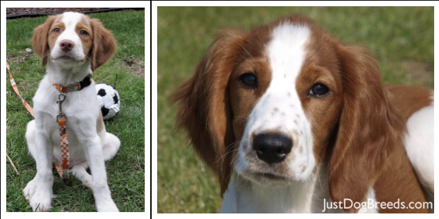
It is not easy to distinguish between the Brittany (left) and the Welsh Springer Spaniel (right) due to similarities in the patterned fur around their eyes

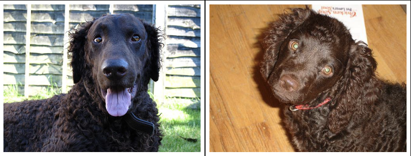
Another pair of dogs, the Curly-coated Retriever (left) and the American Water Spaniel (right), that are difficult to tell apart from the texture of their coats

It may take many weeks or months for a person to learn enough about the physical attributes and unique features of different dog breeds to effectively identify them with a high degree of confidence. It would be interesting to see if a machine learning model can be trained to accomplish the same task in a matter of a few hours. The goal of this project is to use a Convolutional Neural Network (CNN) to train a dog breed classifier across 133 breeds of dogs, using the dogImages dataset, which consists of 8,351 total images split into 133 different categories by dog breed. Everything for this project was done on Amazon Web Services (AWS) and their SageMaker platform as the goal of this project was to further familiarize myself with the AWS ecosystem.

Setup Instructions

The notebook in this repository is intended to be executed using Amazon's SageMaker platform and the following is a brief set of instructions on setting up a managed notebook instance using SageMaker.

Log in to the AWS console and create a notebook instance

Log in to the AWS console and go to the SageMaker dashboard. Click on 'Create notebook instance'. The notebook name can be anything and using ml.t2.medium is a good idea as it is covered under the free tier. To enable GPUs for this particular project, it is recommended to use a ml.p2.xlarge instance. Also it is advised to increase the memory allocation to 15-25GB and to create a Lifecycle Configuration for any required library dependencies. For the role, creating a new role works fine. Using the default options is also okay. Important to note that you need the notebook instance to have access to S3 resources, which it does by default. In particular, any S3 bucket or object with 'sagemaker' in the name is available to the notebook.

Use git to clone the repository into the notebook instance

Once the instance has been started and is accessible, click on 'Open Jupyter' to get to the Jupyter notebook main page. To start, clone this repository into the notebook instance.

Click on the 'new' dropdown menu and select 'terminal'. By default, the working directory of the terminal instance is the home directory, however, the Jupyter notebook hub's root directory is under 'SageMaker'. Enter the appropriate directory and clone the repository as follows.

cd SageMaker
git clone https://github.com/Supearnesh/ml-dog-cnn.git
exit

After you have finished, close the terminal window.

Machine Learning Pipeline

This was the general outline followed for this SageMaker project:

1. Importing the datasets
2. Binary classification
   • a. Detecting humans
   • b. Detecting dogs
3. Convolutional Neural Networks (CNNs)
   • a. Classifying dog breeds from scratch
   • b. Classifying dog breeds using transfer learning
4. Algorithm implementation for images provided as input
5. Model performance testing

Step 1 - Importing the datasets

There are two datasets for this project to be used for this project - dogImages, which contains images of dogs categorized by breed, and lfw, which contains images of humans separated into folders by the individual's name. The dog images dataset has 8,351 total images split into 133 breeds, or categories, of dogs. The data is further broken down into 6,680 images for training, 835 images for validation, and 836 images for testing. The human images dataset has 13,233 total images across 5,749 people. Below are some examples of images from both datasets.

Three separate data loaders are used for training, validation, and test datasets of dog images. Datasets and transforms documentation were helpful in building out these dataloaders.

In addition to separating the data into training, test, and validation sets, the data also needs to be pre-processed. Specifically, all images should be resized to 256 x 256 pixels and then center cropped to 224 x 224 to ensure that they are all uniform in dimensions for the tensor. Also, the red, green, and blue (RGB) color channels should be normalized so that gradient calculations performed by the neural network during training can done more consistently and efficiently. Apart from these items, the images are part of a prepared dataset so there are no abnormalities or inconsistencies that need to be addressed in data pre-processing.

import os
from PIL import Image
from torchvision import datasets
from torchvision import transforms as T
from torch.utils.data import DataLoader

# Set PIL to be tolerant of image files that are truncated.
from PIL import ImageFile
ImageFile.LOAD_TRUNCATED_IMAGES = True

### DONE: Write data loaders for training, validation, and test sets
## Specify appropriate transforms, and batch_sizes
transform = T.Compose([T.Resize(256), T.CenterCrop(224), T.ToTensor(), T.Normalize(mean=[0.485, 0.456, 0.406], std=[0.229, 0.224, 0.225])])

dataset_train = datasets.ImageFolder('dogImages/train', transform=transform)
dataset_valid = datasets.ImageFolder('dogImages/valid', transform=transform)
dataset_test = datasets.ImageFolder('dogImages/test', transform=transform)

loader_train = DataLoader(dataset_train, batch_size=1, shuffle=False)
loader_valid = DataLoader(dataset_valid, batch_size=1, shuffle=False)
loader_test = DataLoader(dataset_test, batch_size=1, shuffle=False)

loaders_scratch = {'train': loader_train, 'valid': loader_valid, 'test': loader_test}

Step 2 - Binary classification

In order to identify the breed of a dog, a model would first need to identify if the image even contains a dog. Once the presence of a dog in the image is confirmed, a multi-class classifier can then begin to determine which breed of dog the image contains. For the scope of this project, 133 breeds were included in the model.

In addition to classifying images of dogs by breed, it would be interesting if the model passed human images as valid input to the classifier as well and found the closest matching breed depending on the human's face. For that purpose, another model can be used to identify if the image contains a human. Once a human has been identified as being present in the image, it can be fed into the multi-class classifier to determine which of the 133 breeds is the closest match.

Part A - Detecting humans

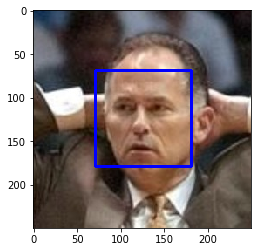
The first model, face_detector, will use OpenCV's implementation of Haar feature-based cascade classifiers to determine if a human face is present, returning true if a face is present, or false if a face is not present in the image.

import cv2
import matplotlib.pyplot as plt
%matplotlib inline

# extract pre-trained face detector
face_cascade = cv2.CascadeClassifier('haarcascades/haarcascade_frontalface_alt.xml')

# load color (BGR) image
img = cv2.imread(human_files[2])
# convert BGR image to grayscale
gray = cv2.cvtColor(img, cv2.COLOR_BGR2GRAY)

# find faces in image
faces = face_cascade.detectMultiScale(gray)

# print number of faces detected in the image
print('Number of faces detected:', len(faces))

# get bounding box for each detected face
for (x,y,w,h) in faces:
    # add bounding box to color image
    cv2.rectangle(img,(x,y),(x+w,y+h),(255,0,0),2)
    
# convert BGR image to RGB for plotting
cv_rgb = cv2.cvtColor(img, cv2.COLOR_BGR2RGB)

# display the image, along with bounding box
plt.imshow(cv_rgb)
plt.show()

Number of faces detected: 1

This implementation of OpenCV achieves a very high face detection in human images (99%) and marginal rates in dog images (10%). An alternative, deep learning approach is the multi-task cascaded convolutional networks (MTCNN) model which is implemented below.

Kaipeng Zhang, Zhanpeng Zhang, Zhifeng Li, and Yu Qiao. Joint Face Detection and Alignment Using Multi-task Cascaded Convolutional Networks. In IEEE Signal Processing Letters, 2016.

import numpy as np
from facenet_pytorch import MTCNN

### DONE: Test performance of another face detection algorithm.
### Feel free to use as many code cells as needed.

# returns "True" if face is detected in image stored at img_path
def face_detector_deep_learning(img_path):
    
    # load image from file
    pixels = plt.imread(img_path)
    
    # create the detector, using default weights
    detector = MTCNN(post_process=False, device='cuda')
    
    # detect faces in the image
    faces, _ = detector.detect(pixels)
    
    return faces is not None

After testing performance of the multi-task convolutional neural network face detection (MTCNN) algorithm, these were the results:

• 100% of the first 100 images in human_files have a detected human face.
• 29% of the first 100 images in dog_files have a detected human face.

The MTCNN implementaiton performs at 100% for human face detection, but also detects faces in more dog images (up 19%). Model performance, however, needs to be weighed against needed functionality. For instance, in a national security application there might be a requirement not to miss any images containing human faces, and in that scenario the MTCNN would be better suited to the task.

Part B - Detecting dogs

The second model, dog_detector, will leverage a pre-trained VGG-16 model to identify if the images contain a dog, returning true if a dog is present, or false if a dog is not present. The VGG-16 model used in this project uses weights that have been trained on ImageNet, a very large, very popular dataset used for image classification and other vision tasks. ImageNet contains over 10 million URLs, each linking to an image containing an object from one of 1000 categories.

from PIL import Image
from torchvision import transforms as T

# Set PIL to be tolerant of image files that are truncated.
from PIL import ImageFile
ImageFile.LOAD_TRUNCATED_IMAGES = True

def VGG16_predict(img_path):
    '''
    Use pre-trained VGG-16 model to obtain index corresponding to 
    predicted ImageNet class for image at specified path
    
    Args:
        img_path: path to an image
        
    Returns:
        Index corresponding to VGG-16 model's prediction
    '''
    
    ## DONE: Complete the function.
    ## Load and pre-process an image from the given img_path
    ## Return the *index* of the predicted class for that 
    
    # load image from file
    img = Image.open(img_path)
    
    # all pre-trained models expect input images normalized in the same way
    # i.e. mini-batches of 3-channel RGB images of shape (3 x H x W)
    # H and W are expected to be at least 224
    transform = T.Compose([T.Resize(256), T.CenterCrop(224), T.ToTensor()])
    transformed_img = transform(img)
    
    # the images have to be loaded in to a range of [0, 1]
    # then normalized using mean = [0.485, 0.456, 0.406] and std = [0.229, 0.224, 0.225]
    normalize = T.Normalize(mean=[0.485, 0.456, 0.406], std=[0.229, 0.224, 0.225])
    normalized_img = normalize(transformed_img)
    
    # model loading
    tensor_img = normalized_img.unsqueeze(0)
    
    # check if CUDA is available
    use_cuda = torch.cuda.is_available()

    # move image tensor to GPU if CUDA is available
    if use_cuda:
        tensor_img = tensor_img.cuda()
        
    prediction = VGG16(tensor_img)

    # move model prediction to CPU if CUDA is available
    if use_cuda:
        prediction = prediction.cpu()
        
    # convert predicted probabilities to class index
    tensor_prediction = torch.argmax(prediction)
    
    # move prediction tensor to CPU if CUDA is available
    if use_cuda:
        tensor_prediction = tensor_prediction.cpu()
    
    predicted_class_index = int(np.squeeze(tensor_prediction.numpy()))
    
    return predicted_class_index # predicted class index

After testing performance of the VGG-16 model, these were the results:

• 0% of the images in human_files have a detected dog.
• 97% of the images in dog_files have a detected dog.

import torch
import torchvision.models as models

### (Optional)
### DONE: Report the performance of another pre-trained network.
### Feel free to use as many code cells as needed.

# define Inception-v3 model
inception = models.inception_v3(pretrained=True)
inception = inception.eval()

# check if CUDA is available
use_cuda = torch.cuda.is_available()

# move model to GPU if CUDA is available
if use_cuda:
    inception = inception.cuda()

def inception_predict(img_path):
    '''
    Use pre-trained Inception-v3 model to obtain index corresponding to 
    predicted ImageNet class for image at specified path
    
    Args:
        img_path: path to an image
        
    Returns:
        Index corresponding to Inception-v3 model's prediction
    '''
    
    ## DONE: Complete the function.
    ## Load and pre-process an image from the given img_path
    ## Return the *index* of the predicted class for that 
    
    # load image from file
    img = Image.open(img_path)
    
    # all pre-trained models expect input images normalized in the same way
    # i.e. mini-batches of 3-channel RGB images of shape (3 x H x W)
    # inception_v3 expects tensors with a size of N x 3 x 299 x 299
    transform = T.Compose([T.Resize(299), T.CenterCrop(299), T.ToTensor()])
    transformed_img = transform(img)
    
    # the images have to be loaded in to a range of [0, 1]
    # then normalized using mean = [0.485, 0.456, 0.406] and std = [0.229, 0.224, 0.225]
    normalize = T.Normalize(mean=[0.485, 0.456, 0.406], std=[0.229, 0.224, 0.225])
    normalized_img = normalize(transformed_img)
    
    # model loading
    tensor_img = normalized_img.unsqueeze(0)
    
    # check if CUDA is available
    use_cuda = torch.cuda.is_available()

    # move image tensor to GPU if CUDA is available
    if use_cuda:
        tensor_img = tensor_img.cuda()
        
    prediction = inception(tensor_img)

    # move model prediction to CPU if CUDA is available
    if use_cuda:
        prediction = prediction.cpu()
        
    # convert predicted probabilities to class index
    tensor_prediction = torch.argmax(prediction)
    
    # move prediction tensor to CPU if CUDA is available
    if use_cuda:
        tensor_prediction = tensor_prediction.cpu()
    
    predicted_class_index = int(np.squeeze(tensor_prediction.numpy()))
    
    return predicted_class_index # predicted class index

An Inception-V3 pretrained model was tested as well and the results were roughly on par with the VGG-16 results:

• 2% of the first 100 images in human_files have a detected dog.
• 98% of the first 100 images in dog_files have a detected dog.

Step 3 - Convolutional Neural Networks (CNNs)

To give a brief overview on the structure of neural networks, they typically consist of connected nodes organized by layers, with an input layer, an output layer and some number of hidden layers in between. At a very high level, the input layer is responsible for taking in data, the hidden layers apply some changes to that data, and the output layer yields the result. There were two CNNs built for this project, one from scratch and another using transfer learning. The goal is to understand the architecture of a CNN better by building one from scratch and then train one using transfer learning to achieve better results. Both CNNs contain an input layer that takes in a pre-processed 3 x 224 x 224 image tensor. The following paper was instrumental for developing a firm understanding of CNNs and for learning strategies to increase performance by decreasing overfitting.

Alex Krizhevsky, Ilya Sutskever, and Geoffrey Hinton. ImageNet Classification with Deep Convolutional Neural Networks. In Proceedings of NIPS, 2012.

Part A - Classifying dog breeds from scratch

This CNN contains five convolutional layers, all normalized and max-pooled, and two fully connected layers with dropout configured at 50% probability. This architecture was modeled after AlexNet. All layers use Rectified Linear Units (ReLUs) for their documented reduction in training times. Even after all of this, the trained model performed quite poorly with the validation loss function severely increasing as the training loss function decreased, a classic sign of bad overfitting. Ultimately, the model managed to identify less than 10% of dog breeds correctly from the test set. Despite several hours' worth of work to combat the overfitting problem, such as trying many iterations of simpler architectures containing only three convolutional layers and increasing the dropout probability of the fully connected layers, the model's performance did not improve. Ultimately, this effort was abandoned in favor of the transfer learning method to create a more proficient model in a lesser amount of time.

Vinod Nair and Geoffrey Hinton. Rectified Linear Units Improve Restricted Boltzmann Machines. In Proceedings of ICML, 2010.

import torch
import torch.nn as nn
import torch.nn.functional as F

# define the CNN architecture
class Net(nn.Module):
    ### DONE: choose an architecture, and complete the class
    def __init__(self):
        super(Net, self).__init__()
        ## Define layers of a CNN
        # convolutional layer (sees 224x224x3 tensor)
        self.conv_01 = nn.Conv2d(in_channels=3, out_channels=32, kernel_size=3, stride=1, padding=1)
        # batch normalization applied to convolutional layer
        self.norm_01 = nn.BatchNorm2d(32)
        # convolutional layer (sees 112x112x32 tensor)
        self.conv_02 = nn.Conv2d(in_channels=32, out_channels=64, kernel_size=3, stride=1, padding=1)
        # batch normalization applied to convolutional layer
        self.norm_02 = nn.BatchNorm2d(64)
        # convolutional layer (sees 56x56x64 tensor)
        self.conv_03 = nn.Conv2d(in_channels=64, out_channels=128, kernel_size=3, stride=1, padding=1)
        # batch normalization applied to convolutional layer
        self.norm_03 = nn.BatchNorm2d(128)
        # convolutional layer pooled (sees 28x28x128 tensor)
        self.conv_04 = nn.Conv2d(in_channels=128, out_channels=256, kernel_size=3, stride=1, padding=1)
        # batch normalization applied to convolutional layer
        self.norm_04 = nn.BatchNorm2d(256)
        # convolutional layer pooled (sees 7x7x256 tensor)
        self.conv_05 = nn.Conv2d(in_channels=256, out_channels=512, kernel_size=3, stride=1, padding=1)
        # batch normalization applied to convolutional layer
        self.norm_05 = nn.BatchNorm2d(512)
        # max pooling layer
        self.pool = nn.MaxPool2d(kernel_size=2, stride=2)
        # linear layer (7 * 7 * 512 -> 500)
        self.fc_01 = nn.Linear(512 * 7 * 7, 4096)
        # linear layer (4096 -> 133)
        self.fc_02 = nn.Linear(4096, 133)
        # dropout layer (p = 0.50)
        self.dropout = nn.Dropout(0.50)
    
    def forward(self, x):
        ## Define forward behavior
        # add sequence of convolutional and max pooling layers
        x = self.pool(F.relu(self.norm_01(self.conv_01(x))))
        x = self.pool(F.relu(self.norm_02(self.conv_02(x))))
        x = self.pool(F.relu(self.norm_03(self.conv_03(x))))
        x = self.pool(F.relu(self.norm_04(self.conv_04(x))))
        x = self.pool(F.relu(self.norm_05(self.conv_05(x))))
        # flatten image input
        x = x.view(-1, 7 * 7 * 512)
        # add dropout layer
        x = self.dropout(x)
        # add first hidden layer, with relu activation function
        x = F.relu(self.fc_01(x))
        # add dropout layer
        x = self.dropout(x)
        # add second hidden layer, with relu activation function
        x = self.fc_02(x)
        return x

#-#-# You do NOT have to modify the code below this line. #-#-#

# create a complete CNN
model_scratch = Net()
print(model_scratch)

# check if CUDA is available
use_cuda = torch.cuda.is_available()

# move tensors to GPU if CUDA is available
if use_cuda: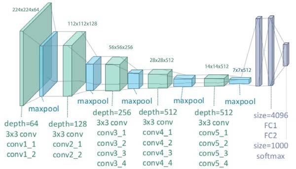
    model_scratch.cuda()

Part B - Classifying dog breeds using transfer learning

In the CNN built using transfer learning, a pre-trained VGG-19 model is used to get much better results than the CNN trained from scratch. Transfer learning involves taking a pre-trained model and using its learnings to get better outcomes for a closely related problem. For instance, a model used to identify images of stop signs could benefit from the learnings of a model trained to identify other street signs. After reading the research paper and looking at the results of the VGG-19 implementation, it seems like a good fit for this project. An illustration of the VGG-19 CNN architecture is included below.

import torchvision.models as models
import torch.nn as nn
import torch

## DONE: Specify model architecture 
model_transfer = models.vgg19(pretrained=True)

for param in model_transfer.parameters():
    param.requires_grad = False

model_transfer.classifier[6] = nn.Linear(4096, 133)

# check if CUDA is available
use_cuda = torch.cuda.is_available()

# move to GPU
if use_cuda:
    model_transfer = model_transfer.cuda()

The pretrained VGG-19 model contains the same architecture as that described by Simonyan and Zisserman in their paper, cited below. The results attained by their model showed great promise for a similar image classification problem and it made sense to reuse the same architecture, only modifying the final fully connected layer to correctly map to the 133 categories being used to classify dog breeds.

Karen Simonyan and Andrew Zisserman. Very Deep Convolutional Networks for Large-scale Image Recognition. In Proceedings of ICLR, 2015.

Step 4 - Pipeline implementation for images provided as input

The end-to-end functionality of this project will employ a multitude of separate components. Any input would first be run through the face_detector and dog_detector functions to determine if the image is of a person or dog. Afterwards, the image would be fed into a CNN to determine the appropriate breed to which the image should belong.

### DONE: Write a function that takes a path to an image as input
### and returns the dog breed that is predicted by the model.

data_transfer = loaders_transfer

# list of class names by index, i.e. a name can be accessed like class_names[0]
class_names = [item[4:].replace("_", " ") for item in data_transfer['train'].dataset.classes]

def predict_breed_transfer(img_path):
    # load the image and return the predicted breed
    global model_transfer
    
    # load image from file
    img = Image.open(img_path)
    
    # all pre-trained models expect input images normalized in the same way
    # i.e. mini-batches of 3-channel RGB images of shape (3 x H x W)
    # H and W are expected to be at least 224
    transform = T.Compose([T.Resize(256), T.CenterCrop(224), T.ToTensor()])
    transformed_img = transform(img)
    
    # the images have to be loaded in to a range of [0, 1]
    # then normalized using mean = [0.485, 0.456, 0.406] and std = [0.229, 0.224, 0.225]
    normalize = T.Normalize(mean=[0.485, 0.456, 0.406], std=[0.229, 0.224, 0.225])
    normalized_img = normalize(transformed_img)
    
    # model loading
    tensor_img = normalized_img.unsqueeze(0)
    
    # check if CUDA is available
    use_cuda = torch.cuda.is_available()
    
    # move image tensor to GPU if CUDA is available
    if use_cuda:
        tensor_img = tensor_img.cuda()
    
    # make prediction by passing image tensor to model
    prediction = model_transfer(tensor_img)
    
    # move model prediction to GPU if CUDA is available
    if use_cuda:
        model_transfer = model_transfer.cuda()
    
    # convert predicted probabilities to class index
    tensor_prediction = torch.argmax(prediction)
    
    # move prediction tensor to CPU if CUDA is available
    if use_cuda:
        tensor_prediction = tensor_prediction.cpu()
    
    predicted_class_index = int(np.squeeze(tensor_prediction.numpy()))
    
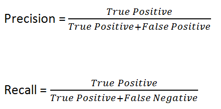
    return class_names[predicted_class_index] # predicted class index

Step 5 - Model performance testing

The final CNN trained using transfer learning performed at a satisfactory level, correctly classifying 60% of the 836 unseen images in the test dataset. This corresponds to a precision of 60% and a recall of 60%. Since this is a multi-class classification problem, every incorrect classification performed by the model is categorized as both a False Positive (FP) and a False Negative (FN). The calculations for precision and recall are included below to illustrate why they are equivalent in this scenario.

While this performance of the model is not particularly extraordinary, it is sufficient for the purposes of this project. While the model is adequate for its purposes, it can be improved by spending more time to perform some additional tuning that is documented earlier in the report. The results from this evaluation can be trusted as the data used for evaluation is data that was unseen by the model during testing. The final model was also thoroughly evaluated on how well the model generalizes to unseen data during training, since a validation set was being used at every training epoch to determine how well the model was performing.

There were several iterations on the CNN in this project, specifically in terms of modifying the number of convolutional layers, configuring dropout, adding max-pooling, and implementing batch normalization. All of these adjustments were made in an effort to lower the degree of overfitting exhibited by the model. Overfitting would imply that the model performs well on the training set but displays noticeable degradation in performance when evaluated against a validation set. This could be observed by noting the divergence of the validation loss function from the training loss function during training; simply put, the validation loss function would begin to increase while the training loss function would continue to decrease, a blatant sign that the model was overfitting. This occurred quite a number of times when training a CNN from scratch, but this behavior was not observed when training the CNN using transfer learning.

There were potential changes that could have been made to improve the performance of the solution in this project: augmenting the training dataset by adding flipped/rotated images would yield a much larger training set and ultimately give better results, experimenting with even more CNN architectures could potentially lead to uncovering a more effective architecture with less overfitting, and utilizing more training epochs, given more time, would both grant the training algorithms more time to converge at the local minimum and help discover patterns in training that could aid in identifying points of improvement. Out of those three, the one that was definitely the easiest to implement, and should have been completed to begin with, was performing data augmentation to the training set with flipped and rotated images. This task alone, would have provided the model with a sizably larger training set to train upon. Using the final solution of this project as a benchmark, it is definitely possible to iterate on it and outperform 60% on dog breed classification.

Important - Deleting the notebook

Always remember to shut down the notebook if it is no longer being used. AWS charges for the duration that a notebook is left running, so if it is left on then there could be an unexpectedly large AWS bill (especially if using a GPU-enabled instance). If allocating considerable space for the notebook (15-25GB), there might be some monthly charges associated with storage as well.