StaVia - Multi-Omic Single-Cell Cartography for Spatial and Temporal Atlases
StaVia (Via 2.0) is our new single-cell trajectory inference method that explores single-cell atlas-scale data and temporal and spatial studies enabled by. In addition to the full functionality of earlier versions, StaVia now offers (check out our preprint for details)
- Integration of metadata (e.g time-series labels, spatial coordinates): Using sequential metadata (temporal labels from longitudinal studies, hierarchical information from phylogenetic trees, spatial distances relevant to spatial omics data) to guide the cartography. Integrating RNA-velocity where applicable.
- Higher Order Random Walks: Leveraging higher order random walks with memory to highlight key end-to-end differentiation pathways along the atlas
- Atlas View: Via 2.0 offers a unique visualization of the predicted trajectory by intuitively merging the cell-cell graph connectivity with the high-resolution of single-cell embeddings. Visit the Gallery to see examples.
- Generalizable and data modality agnostic Via 2.0 still offers all the functionality of Via 1.0 across single-cell data modalities (scRNA-seq, imaging and flow cyometry, scATAC-seq) for types of topologies (disconnected, cyclic, tree) to infer pseudotimes, automated terminal state prediction and automated plotting of temporal gene dynamics along lineages.

StaVia extends the lazy-teleporting walks to higher order random walks with memory to allow better lineage detection, pathway recovery and preservation of global features in terms of computation and visualization. The cartographic approach combining high edge and spatial resolution produces informative and esthetically pleasing visualizations caled the Atlas View.
If you find our work useful, please consider citing our preprint and paper .
Tutorials and videos available on readthedocs with step-by-step code for real and simulated datasets. Tutorials explain how to generate cartographic visualizations for TI, tune parameters, obtain various outputs and also understand the importance of memory. Datasets (anndata h5ad) links are provided below.
✳️ You can start with the The tutorial/Notebook for multifurcating data which shows a step-by-step use case. ✳️
scATAC-seq dataset of Human Hematopoiesis represented by VIA graphs (click image to open interactive graph)

Refer to the Jupiter Notebooks to plot these fine-grained vector fields of the sc-trajectories even when there is no RNA-velocity available.
Tutorials on readthedocs
Please visit our readthedocs for the latest tutorials and videos on usage and installation
| notebook | details | dataset | reference |
|---|---|---|---|
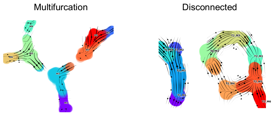
| Multifurcation: Starter Tutorial | 4-leaf simulation | 4-leaf | DynToy |
| Disconnected | disconnected simulation | Disconnected | DynToy |
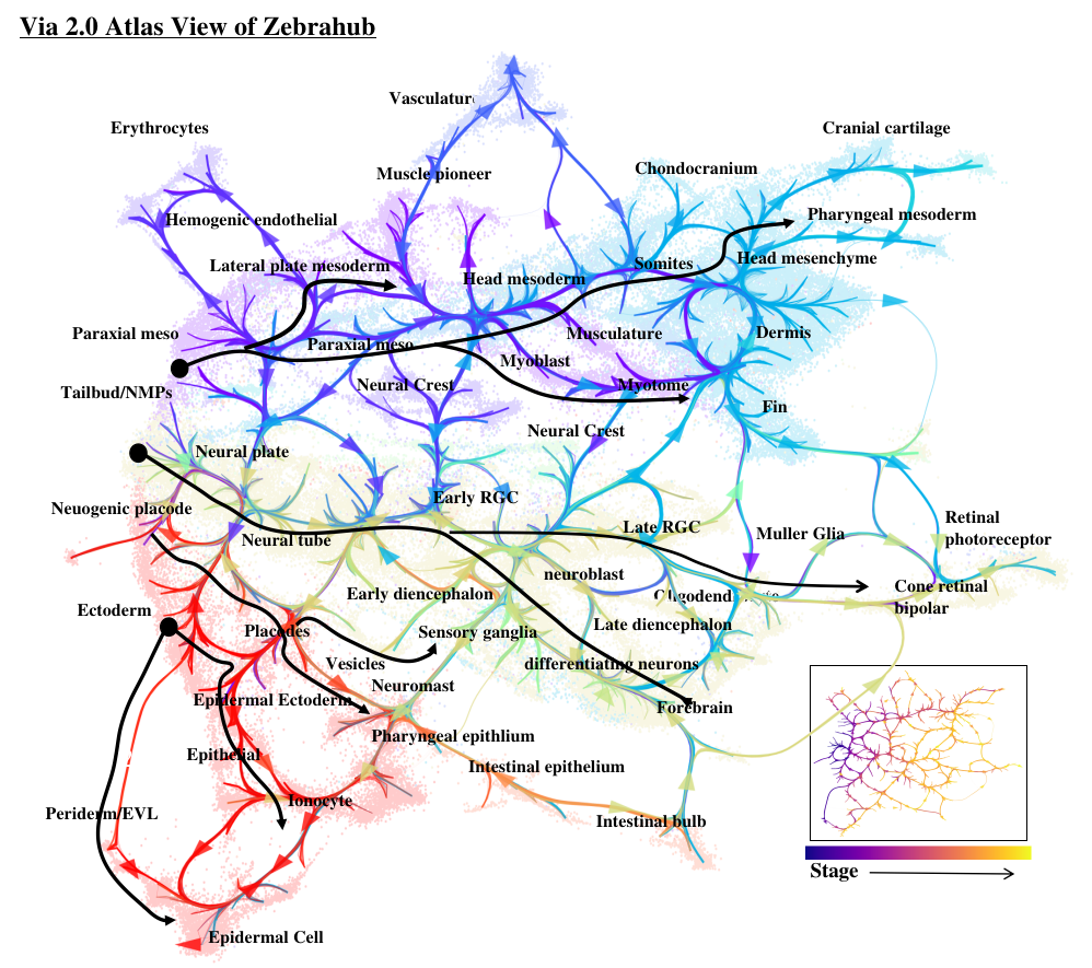
| Zebrafish Gastrulation | Time series of 120,000 cells | Zebrahub | Lange et al. (2023) |
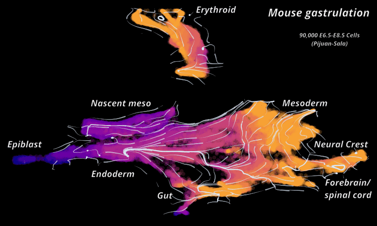
| Mouse Gastrulation | Time series of 90,000 cells | Mouse data | Sala et al. (2019) |
| scRNA-seq Hematopoiesis | Human hematopoiesis (5780 cells) | CD34 scRNA-seq | Setty et al. (2019) |
| FACED image-based | 2036 MCF7 cells in cell cycle | MCF7 FACED | in-house data |
| scATAC-seq Hematopoiesis | Human hematopoiesis | scATAC-seq | Buenrostro et al. (2018) |
Dataset are available in the Datasets folder (smaller files) with larger datasets here.
We recommend setting up a new conda environment and reccomend python version 3.10. Versions 3.8 and 3.9 should also work. You can use the examples below, the Jupyter notebooks and/or the test script to make sure your installation works as expected.
conda create --name ViaEnv python=3.10
pip install pyVIA // tested on linux Ubuntu 16.04 and Windows 10
This usually tries to install hnswlib, produces an error and automatically corrects itself by first installing pybind11 followed by hnswlib. To get a smoother installation, consider installing in the following order after creating a new conda environment:
pip install pybind11
pip install hnswlib
pip install pyVIA
git clone https://github.com/ShobiStassen/VIA.git
python3 setup.py install // cd into the directory of the cloned VIA folder containing setup.py and issue this command
The pie-chart cluster-graph plot does not render correctly for MACs for the time-being. All other outputs are as expected.
conda create --name ViaEnv python=3.10
pip install pybind11
conda install -c conda-forge hnswlib
pip install pyVIA
If the pip install doesn't work, it usually suffices to first install all the requirements (using pip) and subsequently install VIA (also using pip). Note that on Windows if you do not have Visual C++ (required for hnswlib) you can install using this link .
pip install pybind11, hnswlib, igraph, leidenalg>=0.7.0, umap-learn, numpy>=1.17, scipy, pandas>=0.25, sklearn, termcolor, pygam, phate, matplotlib,scanpy
pip install pyVIA
All examples and tests have been run on Linux and MAC OS. We find there are somtimes small modifications required to run on a Windows OS (see below). Windows requires minor modifications in calling the code due to the way multiprocessing works in Windows compared to Linux:
#when running from an IDE you need to call the function in the following way to ensure the parallel processing works:
import os
import pyVIA.core as via
f= os.path.join(r'C:\Users\...\Documents'+'\\')
def main():
    via.main_Toy(ncomps=10, knn=30,dataset='Toy3', random_seed=2,foldername= f)
if __name__ =='__main__':
    main()

#when running directly from terminal:
import os
import pyVIA.core as via
f= os.path.join(r'C:\Users\...\Documents'+'\\')
via.main_Toy(ncomps=10, knn=30,dataset='Toy3', random_seed=2,foldername= f)
| Input Parameter for class VIA | Description |
|---|---|
data |
(numpy.ndarray) n_samples x n_features. When using via_wrapper(), data is ANNdata object that has a PCA object adata.obsm['X_pca'][:, 0:ncomps] and ncomps is the number of components that will be used. |
true_label |
(list) 'ground truth' annotations or placeholder |
memory |
(float) default =5 higher memory means lineage pathways that deviate less from predecessors |
times_series |
(bool) default=False. whether or not sequential augmentation of the TI graph will be done based on time-series labels |
time_series_labels |
(list) list (length n_cells) of numerical values corresponding to sequential/chronological/hierarchical sequence |
knn |
(optional, default = 30) number of K-Nearest Neighbors for HNSWlib KNN graph |
root_user |
root_user should be provided as a list containing roots corresponding to index (row number in cell matrix) of root cell. For most trajectories this is of the form [53] where 53 is the index of a sensible root cell, for multiple disconnected trajectories an arbitrary list of cells can be provided [1,506,1100], otherwise VIA arbitratily chooses cells. If the root cells of disconnected trajectories are known in advance, then the cells should be annotated with similar syntax to that of Example Dataset in Disconnected Toy Example 1b. |
dist_std_local |
(optional, default = 1) local pruning threshold for PARC clustering stage: the number of standard deviations above the mean minkowski distance between neighbors of a given node. the higher the parameter, the more edges are retained |
edgepruning_clustering_resolution |
(optional, default = 0.15) global level graph pruning for PARC clustering stage. 0.1-1 provide reasonable pruning. higher value means less pruning. e.g. a value of 0.15 means all edges that are above mean(edgeweight)-0.15*std(edge-weights) are retained. We find both 0.15 and 'median' to yield good results resulting in pruning away ~ 50-60% edges |
too_big_factor |
(optional, default = 0.4) if a cluster exceeds this share of the entire cell population, then the PARC will be run on the large cluster |
cluster_graph_pruning |
(optional, default =0.15) To retain more edges/connectivity in the graph underlying the trajectory computations, increase the value |
edgebundle_pruning |
(optional) default value is the same as cluster_grap_pruning. Only impacts the visualized edges, not the underlying edges for computation and TI |
x_lazy |
(optional, default = 0.95) 1-x = probability of staying in same node (lazy). Values between 0.9-0.99 are reasonable |
alpha_teleport |
(optional, default = 0.99) 1-alpha is probability of jumping. Values between 0.95-0.99 are reasonable unless prior knowledge of teleportation |
distance |
(optional, default = 'l2' euclidean) 'ip','cosine' |
random_seed |
(optional, default = 42) The random seed to pass to Leiden |
pseudotime_threshold_TS |
(optional, default = 30) Percentile threshold for potential node to qualify as Terminal State |
resolution_parameter |
(optional, default = 1) Uses ModuliartyVP and RBConfigurationVertexPartition |
preserve_disconnected |
(optional, default = True) If you do not think there should be any disconnected trajectories, set this to False |
| Attributes | Description |
|---|---|
labels |
(list) length n_samples of corresponding cluster labels |
single_cell_pt_markov |
(list) computed pseudotime |
embedding |
2d array representing a computed embedding |
single_cell_bp |
(array) computed single cell branch probabilities (lineage likelihoods). n_cells x n_terminal states. The columns each correspond to a terminal state, in the same order presented in the'terminal_clusters' attribute |
terminal clusters |
(list) terminal clusters found by VIA |
full_neighbor_array |
full_neighbor_array=v0.full_neighbor_array. KNN graph from first pass of via - neighbor array |
full_distance_array |
full_distance_array=v0.full_distance_array. KNN graph from first pass of via - edge weights |
ig_full_graph |
ig_full_graph=v0.ig_full_graph igraph of the KNN graph from first pass of via |
csr_full_graph |
csr_full_graph. If time_series is true, this is sequentially augmented. |
csr_array_locally_pruned |
csr_array_locally_pruned=v0.csr_array_locally_pruned. CSR matrix of the locally pruned KNN graph |