Dimensionality Reduction Techniques

Overview:

With the availability of high-performance CPUs and GPUs, it is pretty much possible to solve every regression, classification, clustering, and other related problems using machine learning and deep learning models. However, there are still various portions that cause performance bottlenecks while developing such models. A large number of features in the dataset are one of the major factors that affect both the training time as well as the accuracy of machine learning models.
The Curse of Dimensionality is termed by mathematician R. Bellman in his book “Dynamic Programming” in 1957. According to him, the curse of dimensionality is the problem caused by the exponential increase in volume associated with adding extra dimensions to Euclidean space. In machine learning, “dimensionality” simply refers to the number of features (i.e. input variables) in your dataset.

While the performance of any machine learning model increases if we add additional features/dimensions, at some point a further insertion leads to performance degradation that is when the number of features is very large commensurate with the number of observations in your dataset, several linear algorithms strive hard to train efficient models. This is called the “Curse of Dimensionality”.
The curse of dimensionality basically means that the error increases with the increase in the number of features. It refers to the fact that algorithms are harder to design in high dimensions and often have a running time exponential in the dimensions.

We need a better way to deal with such a high dimensional data so that we can quickly extract patterns and insights from it. So how do we approach such a dataset? Using dimensionality reduction techniques, indeed. We can use this concept to reduce the number of features in our dataset without having to lose much information and keep (or improve) the model’s performance.
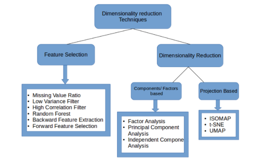
Dimensionality reduction is a set of techniques that studies how to shrivel the size of data while preserving the most important information and further eliminating the curse of dimensionality. It plays an important role in the performance of classification and clustering problems.

Various techniques used for dimensionality reduction:

Implementation:

Libraries: NumPy pandas tensorflow matplotlib sklearn seaborn

High Correlation Filter:

High correlation between two variables means they have similar trends and are likely to carry similar information. This can bring down the performance of some models drastically.
As a general guideline, we should keep those variables which show a decent or high correlation with the target variable.

Random Forest:

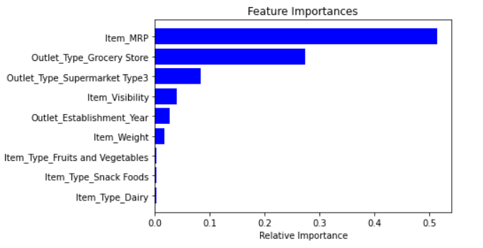
Random Forest is one of the most widely used algorithms for feature selection. It comes packaged with in-built feature importance so you don’t need to program that separately. This helps us select a smaller subset of features.

from sklearn.ensemble import RandomForestRegressor
df=df.drop(['Item_Identifier', 'Outlet_Identifier'], axis=1)
model = RandomForestRegressor(random_state=1, max_depth=10)
df=pd.get_dummies(df)
model.fit(df,train.Item_Outlet_Sales)

features = df.columns
importances = model.feature_importances_

Backward feature elimination

• We first take all the n variables present in our dataset and train the model using them
• We then calculate the performance of the model
• Now, we compute the performance of the model after eliminating each variable (n times), i.e., we drop one variable every time and train the model on the remaining n-1 variables
• We identify the variable whose removal has produced the smallest (or no) change in the performance of the model, and then drop that variable

Forward feature elimination

This is the opposite process of the Backward Feature Elimination we saw above. Instead of eliminating features, we try to find the best features which improve the performance of the model.

Both Backward Feature Elimination and Forward Feature Selection are time consuming and computationally expensive.

Factor Analysis:

In the Factor Analysis technique, variables are grouped by their correlations, i.e., all variables in a particular group will have a high correlation among themselves, but a low correlation with variables of other group(s). Here, each group is known as a factor. These factors are small in number as compared to the original dimensions of the data. However, these factors are difficult to observe.

Dataset:

Indentify the apparels

images = [cv2.imread(file) for file in glob('train_/train/*.png')]
images = np.array(images)
image = []
for i in range(0,60000):
    img = images[i].flatten()
    image.append(img)
image = np.array(image)
train = pd.read_csv("train_/train.csv")     # Give the complete path of your train.csv file
feat_cols = [ 'pixel'+str(i) for i in range(image.shape[1]) ]
df = pd.DataFrame(image,columns=feat_cols)
df['label'] = train['label'

# decompose the data using factor Analysis
from sklearn.decomposition import FactorAnalysis
FA = FactorAnalysis(n_components = 3).fit_transform(df[feat_cols].values)

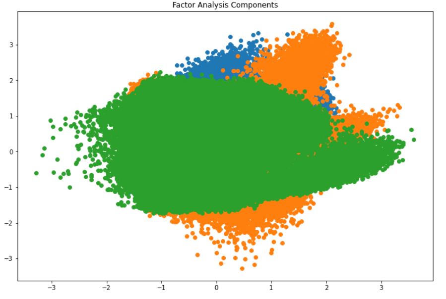
Here, the x-axis and y-axis represent the values of decomposed factors.
It is hard to observe these factors individually but we have been able to reduce the dimensions of our data successfully.

Principal Component Analysis (PCA):

Principal Component Analysis(PCA) is one of the most popular linear dimension reduction algorithms. It is a projection based method that transforms the data by projecting it onto a set of orthogonal(perpendicular) axes. PCA is a technique which helps us in extracting a new set of variables from an existing large set of variables. These newly extracted variables are called Principal Components.

from sklearn.decomposition import PCA
pca = PCA(n_components=4)
pca_result = pca.fit_transform(df[feat_cols].values)

Let’s visualize how much variance has been explained using these 4 components. We will use explained_variance_ratio_ to calculate the same.

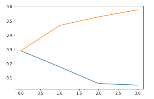
In the above graph, the blue line represents component-wise explained variance while the orange line represents the cumulative explained variance. We are able to explain around 60% variance in the dataset using just four components.

Checkout more details about PCA in the Notebook

Independent Component Analysis:

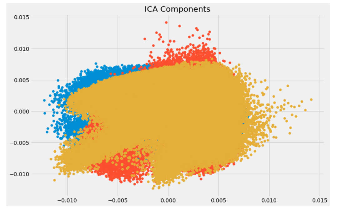
Independent Component Analysis (ICA) is based on information-theory and is also one of the most widely used dimensionality reduction techniques. The major difference between PCA and ICA is that PCA looks for uncorrelated factors while ICA looks for independent factors. This algorithm assumes that the given variables are linear mixtures of some unknown latent variables. It also assumes that these latent variables are mutually independent, i.e., they are not dependent on other variables and hence they are called the independent components of the observed data.

from sklearn.decomposition import FastICA 
ICA = FastICA(n_components=3, random_state=12) 
X=ICA.fit_transform(df[feat_cols].values)

Methods based on Projection:

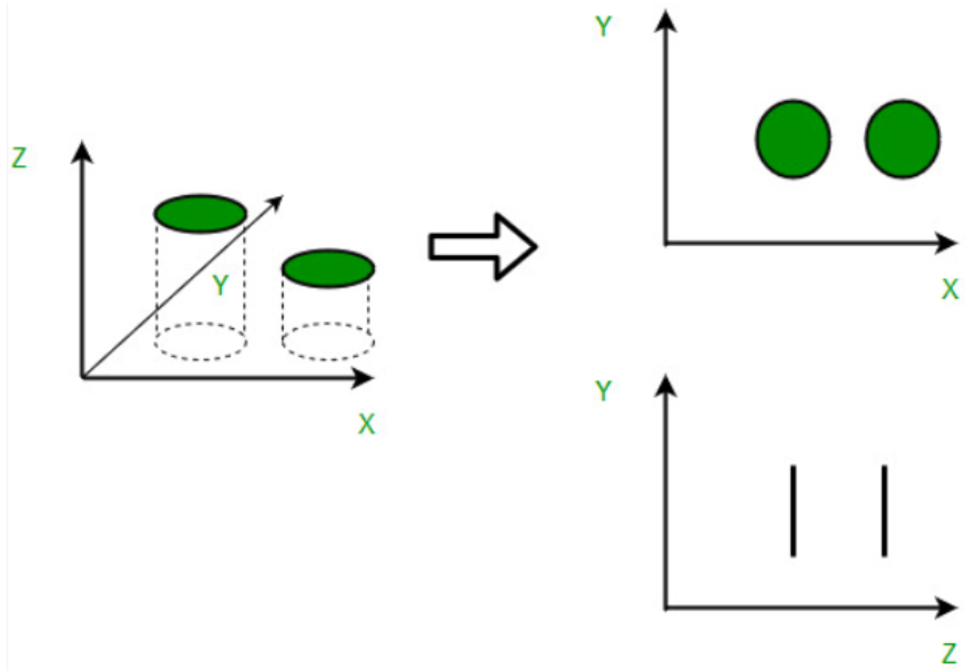
In projection techniques, multi-dimensional data is represented by projecting its points onto a lower-dimensional space.
know more about this method here

from sklearn import manifold 
trans_data = manifold.Isomap(n_neighbors=5, n_components=3, n_jobs=-1).fit_transform(df[feat_cols][:6000].values)

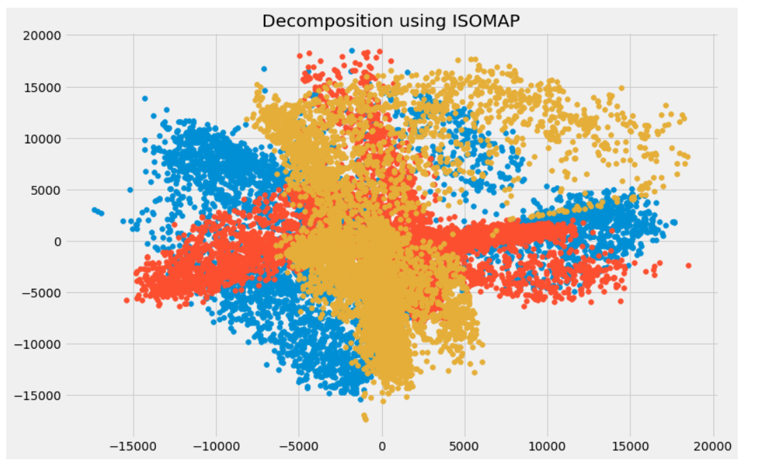
Correlation between the components is very low.

t-Distributed Stochastic Neighbor Embedding (t-SNE):

PCA is a good choice for dimensionality reduction and visualization for datasets with a large number of variables. But, for searching the patterns nonlinearly, we need more advanced technique. t-SNE is one such technique. t-SNE is one of the few algorithms which is capable of retaining both local and global structure of the data at the same time. It calculates the probability similarity of points in high dimensional space as well as in low dimensional space.

from sklearn.manifold import TSNE 
tsne = TSNE(n_components=3, n_iter=300).fit_transform(df[feat_cols][:6000].values)

Here you can clearly see the different components that have been transformed using the powerful t-SNE technique.

Uniform Manifold Approximation and Projection (UMAP):

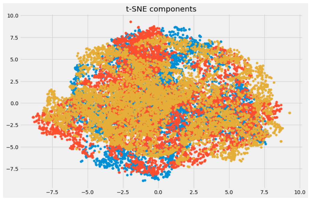
t-SNE works very well on large datasets but it also has it’s limitations, such as loss of large-scale information, slow computation time, and inability to meaningfully represent very large datasets. Uniform Manifold Approximation and Projection (UMAP) is a dimension reduction technique that can preserve as much of the local, and more of the global data structure as compared to t-SNE, with a shorter runtime.

import umap
umap_data = umap.UMAP(n_neighbors=5, min_dist=0.3, n_components=3).fit_transform(df[feat_cols][:6000].values)

The dimensions have been reduced and we can visualize the different transformed components. There is very less correlation between the transformed variables.
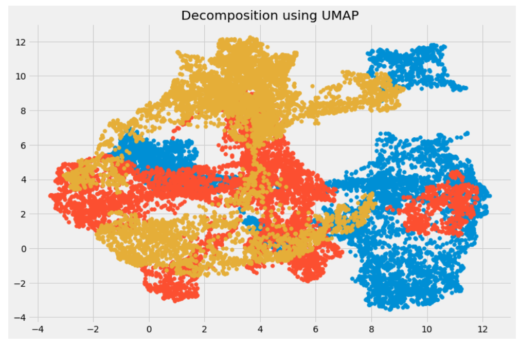
We can see that the correlation between the components obtained from UMAP is quite less as compared to the correlation between the components obtained from t-SNE. Hence, UMAP tends to give better results.

References:

Dimensionality Reduction
Dimensionality Reduction Techniques
t-SNE
UMAP

Feedback

If you have any feedback, please reach out at pradnyapatil671@gmail.com

🚀 About Me

Hi, I'm Pradnya! 👋

I am an AI Enthusiast and Data science & ML practitioner