- Let's talk about Differential Derivative and Partial Derivative
- Gradient Descent
- Overview
-
To better understand the difference between the differential and derivative of a function. You need to understand the concept of a function.
-
A function is one of the basic concepts in mathematics that defines a relationship between a set of inputs and a set of possible outputs where each input is related to one output. Where Input variables are the independent variables and the other which is output variable is the dependent variable.
-
Take for example the statement " 'y' is a function of
$x$ i.e y=$f(x)$ which means something related to y is directly related to x by some formula. -
The Calculus as a tool defines the derivative of a function as the limit of a particular kind.
It is one of the fundamentals divisions of calculus, along with integral calculus. It is a subfield of calculus that deals with infinitesimal change in some varying quantity. The world we live in is full of interrelated quantities that change periodically.
For example, the area of a circular body which changes as the radius changes or a projectile which changes with the velocity. These changing entities, in mathematical terms, are called as variables and the rate of change of one variable with respect to another is a derivative. And the equation which represents the relationship between these variables is called a differential equation.
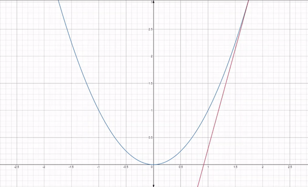
The derivative of a function represents an instantaneous rate of change in the value of a dependent variable with respect to the change in value of the independent variable. It’s a fundamental tool of calculus which can also be interpreted as the slope of the tangent line. It measures how steep the graph of a function is at some given point on the graph.
-
It measures how steep the graph of a function is at some given point on the graph
-
Equations which define relationship between there variables and their derivatives are called Differential Equations.
-
Differentiation is the process of finding a derivative.
-
The derivative of a function is the rate of change of the output value with respect to its input value, where as differential is the actual change of function.
-
Differentials are represented as
$d_x$ ,$d_y$ ,$d_t$ , and so on, where$d_x$ represents a small change in$x$ , etc. -
When comparing changes in related quantities where y is the function of x, the differential
$d_y$ is written as y =$f$ (x) -
$\frac{d_y}{d_x}=f(x)$ -
The derivative of a function is the slope of the function at any point and is written as
$\frac{d}{d_x}$ . -
For example, the derivative of
$sin(x)$ can be written as$\frac{d_{sin(x)}}{d_x}=cos(x)$
Partial differentiation is used to differentiate mathematical functions having more than one variable in them. In ordinary differentiation, we find derivative with respect to one variable only, as function contains only one variable. So partial differentiation is more general than ordinary differentiation. Partial differentiation is used for finding maxima and minima in optimization problems.
It is a derivative where we hold some independent variable as constant and find derivative with respect to another independent variable.
For example, suppose we have an equation of a curve with X and Y coordinates in it as 2 independent variables. To find the slope in the direction of X, while keeping Y fixed, we will find the partial derivative. Similarly, we can find the slope in the direction of Y (keeping X as Fixed).
Example: consider
In ordinary differentition the same equation goes like


- Optimization is the core of every machine learning algorithm
To explain Gradient Descent I’ll use the classic mountaineering example.
Suppose you are at the top of a mountain, and you have to reach a lake which is at the lowest point of the mountain (a.k.a valley). A twist is that you are blindfolded and you have zero visibility to see where you are headed. So, what approach will you take to reach the lake?
The best way is to check the ground near you and observe where the land tends to descend. This will give an idea in what direction you should take your first step. If you follow the descending path, it is very likely you would reach the lake.
To represent this graphically, notice the below graph.

Let us now map this scenario in mathematical terms.
Suppose we want to find out the best parameters (θ1) and (θ2) for our learning algorithm. Similar to the analogy above, we see we find similar mountains and valleys when we plot our “cost space”. Cost space is nothing but how our algorithm would perform when we choose a particular value for a parameter.
So on the y-axis, we have the cost J(θ) against our parameters θ1 and θ2 on x-axis and z-axis respectively. Here, hills are represented by red region, which have high cost, and valleys are represented by blue region, which have low cost.


It is defind as the measurement of difference of error between actual values and expected values at the current position
The slight difference between the loss fucntion and the cost function is about the error within the training of machine learning models, as loss function refers to the errors of one training example, while a cost function calculates the average error across on entire training set.
-
Gradient descent is an optimization algorithm that works iteratively to find the model parameters with minimal cost or error values. If we go through a formal definition of Gradient descent
-
Gradient descent is a first-order iterative optimization algorithm for finding a local minimum of a differentiable function.Gradient descent is an optimization algorithm used to optimize neural networks and many other machine learning algorithms. Our main goal in optimization is to find the local minima, and gradient descent helps us to take repeated steps in the direction opposite of the gradient of the function at the current point. This method is commonly used in machine learning (ML) and deep learning (DL) to minimize a cost/loss function
Mean Squared Error- The Mean Squared Error (MSE) is perhaps the simplest and most common loss function, often taught in introductory Machine Learning courses. To calculate the MSE, you take the difference between your model’s predictions and the ground truth, square it, and average it out across the whole dataset.
The MSE will never be negative, since we are always squaring the errors. The MSE is formally defined by the following equation:

Where N is the number of samples we are testing against.


Advantage: The MSE is great for ensuring that our trained model has no outlier predictions with huge errors, since the MSE puts larger weight on theses errors due to the squaring part of the function.
Disadvantage: If our model makes a single very bad prediction, the squaring part of the function magnifies the error. Yet in many practical cases we don’t care much about these outliers and are aiming for more of a well-rounded model that performs good enough on the majority.
Absolute Error loss
The Mean Absolute Error (MAE) is only slightly different in definition from the MSE, but interestingly provides almost exactly opposite properties! To calculate the MAE, you take the difference between your model’s predictions and the ground truth, apply the absolute value to that difference, and then average it out across the whole dataset.
The MAE, like the MSE, will never be negative since in this case we are always taking the absolute value of the errors. The MAE is formally defined by the following equation:


Advantage: The beauty of the MAE is that its advantage directly covers the MSE disadvantage. Since we are taking the absolute value, all of the errors will be weighted on the same linear scale. Thus, unlike the MSE, we won’t be putting too much weight on our outliers and our loss function provides a generic and even measure of how well our model is performing.
Disadvantage: If we do in fact care about the outlier predictions of our model, then the MAE won’t be as effective. The large errors coming from the outliers end up being weighted the exact same as lower errors. This might results in our model being great most of the time, but making a few very poor predictions every so-often.
Huber Loss
Now we know that the MSE is great for learning outliers while the MAE is great for ignoring them. But what about something in the middle?
Consider an example where we have a dataset of 100 values we would like our model to be trained to predict. Out of all that data, 25% of the expected values are 5 while the other 75% are 10.
An MSE loss wouldn’t quite do the trick, since we don’t really have “outliers”; 25% is by no means a small fraction. On the other hand we don’t necessarily want to weight that 25% too low with an MAE. Those values of 5 aren’t close to the median (10 — since 75% of the points have a value of 10), but they’re also not really outliers.
Our solution?
The Huber Loss Function.
The Huber Loss offers the best of both worlds by balancing the MSE and MAE together. We can define it using the following piecewise function:

What this equation essentially says is: for loss values less than delta, use the MSE; for loss values greater than delta, use the MAE. This effectively combines the best of both worlds from the two loss functions!
Using the MAE for larger loss values mitigates the weight that we put on outliers so that we still get a well-rounded model. At the same time we use the MSE for the smaller loss values to maintain a quadratic function near the centre.
This has the effect of magnifying the loss values as long as they are greater than 1. Once the loss for those data points dips below 1, the quadratic function down-weights them to focus the training on the higher-error data points.

Cross Entropy

If you are training a binary classifier, chances are you are using binary cross-entropy / log loss as your loss function.
A Simple Classification Problem Let’s start with 10 random points:
x = [-2.2, -1.4, -0.8, 0.2, 0.4, 0.8, 1.2, 2.2, 2.9, 4.6]
This is our only feature: x.

Now, let’s assign some colors to our points: red and green. These are our labels

So, our classification problem is quite straightforward: given our feature x, we need to predict its label: red or green.
Since this is a binary classification, we can also pose this problem as: “is the point green” or, even better, “what is the probability of the point being green”? Ideally, green points would have a probability of 1.0 (of being green), while red points would have a probability of 0.0 (of being green).
In this setting, green points belong to the positive class (YES, they are green), while red points belong to the negative class (NO, they are not green).
If we fit a model to perform this classification, it will predict a probability of being green to each one of our points. Given what we know about the color of the points, how can we evaluate how good (or bad) are the predicted probabilities? This is the whole purpose of the loss function! It should return high values for bad predictions and low values for good predictions.
For a binary classification like our example, the typical loss function is the binary cross-entropy / log loss.
- Loss Function: Binary Cross-Entropy / Log Loss
If you look this loss function up, this is what you’ll find:

where y is the label (1 for green points and 0 for red points) and p(y) is the predicted probability of the point being green for all N points.
Reading this formula, it tells you that, for each green point (y=1), it adds log(p(y)) to the loss, that is, the log probability of it being green. Conversely, it adds log(1-p(y)), that is, the log probability of it being red, for each red point (y=0). Not necessarily difficult, sure, but no so intuitive too…
But, before going into more formulas, let me show you a visual representation of the formula above…
Computing the Loss — the visual way First, let’s split the points according to their classes, positive or negative, like the figure below:

Now, let’s train a Logistic Regression to classify our points. The fitted regression is a sigmoid curve representing the probability of a point being green for any given x . It looks like this:

Then, for all points belonging to the positive class (green), what are the predicted probabilities given by our classifier? These are the green bars under the sigmoid curve, at the x coordinates corresponding to the points.

OK, so far, so good! What about the points in the negative class? Remember, the green bars under the sigmoid curve represent the probability of a given point being green. So, what is the probability of a given point being red? The red bars ABOVE the sigmoid curve, of course :-)

Putting it all together, we end up with something like this:

The bars represent the predicted probabilities associated with the corresponding true class of each point!
OK, we have the predicted probabilities… time to evaluate them by computing the binary cross-entropy / log loss!
These probabilities are all we need, so, let’s get rid of the x axis and bring the bars next to each other:

Well, the hanging bars don’t make much sense anymore, so let’s reposition them:

Since we’re trying to compute a loss, we need to penalize bad predictions, right? If the probability associated with the true class is 1.0, we need its loss to be zero. Conversely, if that probability is low, say, 0.01, we need its loss to be HUGE!
It turns out, taking the (negative) log of the probability suits us well enough for this purpose (since the log of values between 0.0 and 1.0 is negative, we take the negative log to obtain a positive value for the loss).
The plot below gives us a clear picture —as the predicted probability of the true class gets closer to zero, the loss increases exponentially:

Fair enough! Let’s take the (negative) log of the probabilities — these are the corresponding losses of each and every point.
Finally, we compute the mean of all these losses.

Voilà! We have successfully computed the binary cross-entropy / log loss of this toy example. It is 0.3329!
- Distribution
Let’s start with the distribution of our points. Since y represents the classes of our points (we have 3 red points and 7 green points), this is what its distribution, let’s call it q(y), looks like:

- Entropy
Entropy is a measure of the uncertainty associated with a given distribution q(y).
What if all our points were green? What would be the uncertainty of that distribution? ZERO, right? After all, there would be no doubt about the color of a point: it is always green! So, entropy is zero!
On the other hand, what if we knew exactly half of the points were green and the other half, red? That’s the worst case scenario, right? We would have absolutely no edge on guessing the color of a point: it is totally random! For that case, entropy is given by the formula below (we have two classes (colors)— red or green — hence,

For every other case in between, we can compute the entropy of a distribution, like our q(y), using the formula below, where C is the number of classes:

So, if we know the true distribution of a random variable, we can compute its entropy. But, if that’s the case, why bother training a classifier in the first place? After all, we KNOW the true distribution…
But, what if we DON’T? Can we try to approximate the true distribution with some other distribution, say, p(y)? Sure we can! :-)
- Cross-Entropy
Let’s assume our points follow this other distribution p(y). But we know they are actually coming from the true (unknown) distribution q(y), right?
If we compute entropy like this, we are actually computing the cross-entropy between both distributions:

If we, somewhat miraculously, match p(y) to q(y) perfectly, the computed values for both cross-entropy and entropy will match as well.
Since this is likely never happening, cross-entropy will have a BIGGER value than the entropy computed on the true distribution.

It turns out, this difference between cross-entropy and entropy has a name…
- Kullback-Leibler Divergence
The Kullback-Leibler Divergence,or “KL Divergence” for short, is a measure of dissimilarity between two distributions:

This means that, the closer p(y) gets to q(y), the lower the divergence and, consequently, the cross-entropy, will be.
So, we need to find a good p(y) to use… but, this is what our classifier should do, isn’t it?! And indeed it does! It looks for the best possible p(y), which is the one that minimizes the cross-entropy.
- Loss Function
During its training, the classifier uses each of the N points in its training set to compute the cross-entropy loss, effectively fitting the distribution p(y)! Since the probability of each point is 1/N, cross-entropy is given by:

Remember Figures 6 to 10 above? We need to compute the cross-entropy on top of the probabilities associated with the true class of each point. It means using the green bars for the points in the positive class (y=1) and the red hanging bars for the points in the negative class (y=0) or, mathematically speaking:

The final step is to compute the average of all points in both classes, positive and negative:

Finally, with a little bit of manipulation, we can take any point, either from the positive or negative classes, under the same formula:

Voilà! We got back to the original formula for binary cross-entropy / log loss :-)
Binary Cross Entropy for Multi-Class classification If you are dealing with a multi-class classification problem you can calculate the Log loss in the same way. Just use the formula given below.

Multi-Class Cross Entropy


- Categorical crossentropy Categorical crossentropy is a loss function that is used in multi-class classification tasks. These are tasks where an example can only belong to one out of many possible categories, and the model must decide which one. Formally, it is designed to quantify the difference between two probability distributions.

Categorical crossentropy math The categorical crossentropy loss function calculates the loss of an example by computing the following sum:

Sigmoid
It squashes a vector in the range (0, 1). It is applied independently to each element of


Softmax
Softmax it’s a function, not a loss. It squashes a vector in the range (0, 1) and all the resulting elements add up to 1. It is applied to the output scores


Loss function vs Cost function Most people confuse loss function and cost function. let’s understand what is loss function and cost function. Cost function and Loss function are synonymous and used interchangeably but they are different.
Loss Function:
A loss function/error function is for a single training example/input.
Cost Function:
A cost function, on the other hand, is the average loss over the entire training dataset.

The loss function quantifies how much a model \boldsymbol{f}‘s prediction \boldsymbol{\hat{y} \equiv f(\mathbf{x})} deviates from the ground truth \boldsymbol{y \equiv y(\mathbf{x})} for one particular object \mathbf{x}. So, when we calculate loss, we do it for a single object in the training or test sets.
There are many different loss functions we can choose from, and each has its advantages and shortcomings. In general, any distance metric defined over the space of target values can act as a loss function.
Example: the Square and Absolute Losses in Regression Very often, we use the square(d) error as the loss function in regression problems:

For instance, let’s say that our model predicts a flat’s price (in thousands of dollars) based on the number of rooms, area (m^2), floor, and the neighborhood in the city (A or B). Let’s suppose that its prediction for \mathbf{x} = \begin{bmatrix} 4, 70, 1, A \end{bmatrix} is USD 110k. If the actual selling price is USD 105k, then the square loss is:

Another loss function we often use for regression is the absolute loss:

In our example with apartment prices, its value will be:

Choosing the loss function isn’t an easy task. Through cost, loss plays a critical role in fitting a model.
The term cost is often used as synonymous with loss. However, some authors make a clear difference between the two. For them, the cost function measures the model’s error on a group of objects, whereas the loss function deals with a single data instance.
So, if L is our loss function, then we calculate the cost function by aggregating the loss L over the training, validation, or test data \mathcal{D}= \left{ (\mathbf{x}i, y_i) \right}{i=1}^{n}. For example, we can compute the cost as the mean loss:

But, nothing stops us from using the median, the summary statistic less sensitive to outliers:

The cost functions serve two purposes. First, its value for the test data estimates our model’s performance on unseen objects. That allows us to compare different models and choose the best. Second, we use it to train our models.
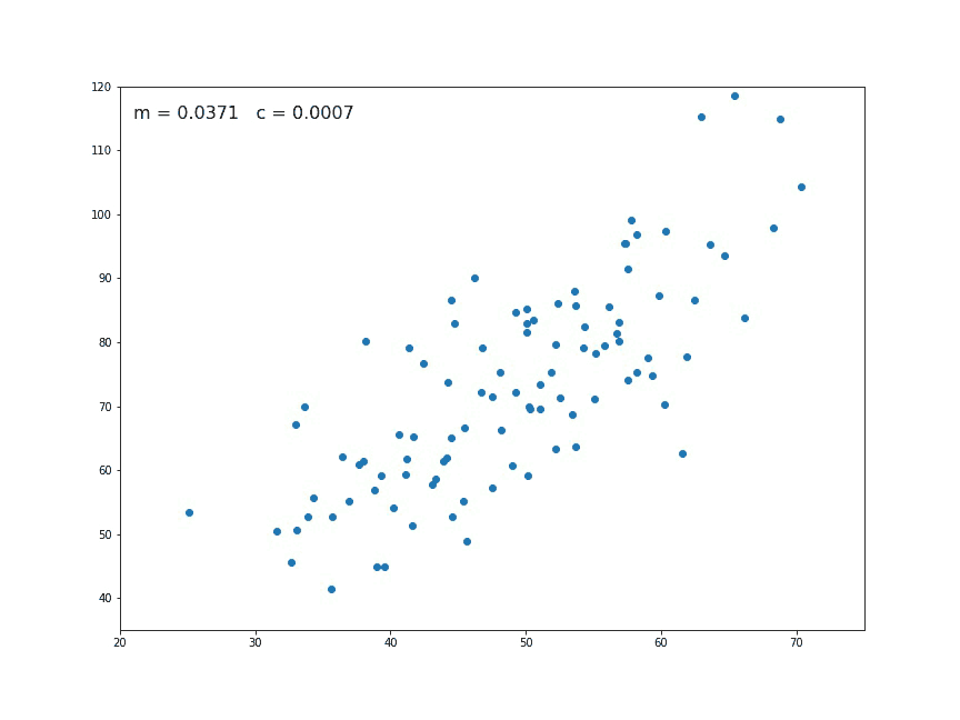
A straight line is represented by using the formula y = m$x$ + c
- y is the dependent variable
-
$x$ is independent variable - m is the slope of the line
- c is the y intercept


We will use the Mean Squared Error function to calculate the loss. There are three steps in this function:
- Find the difference between the actual y and predicted y value(y = mx + c), for a given x.
- Square this difference.
- Find the mean of the squares for every value in X.

Here yᵢ is the actual value and ȳᵢ is the predicted value. Lets substitute the value of ȳᵢ:

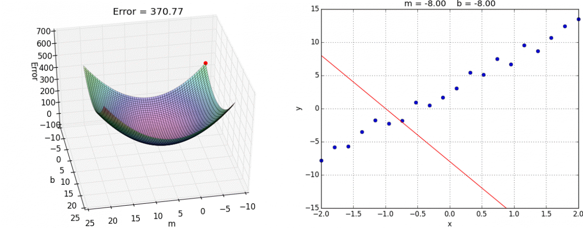
The loss function helps to increase and improve machine learning efficiency by providing feedback to the model, so that it can minimize error and find the global minima. Further, it continuously iterates along the direction of the negative gradient until the cost function approaches zero.
Calculating the partial derivative of the cost function with respect to slope (m), let the partial derivative of the cost function with respect to m be
Let’s try applying gradient descent to m and c and approach it step by step:
- Initially let m = 0 and c = 0. Let L be our learning rate. This controls how much the value of m changes with each step. L could be a small value like 0.0001 for good accuracy.
- Calculate the partial derivative of the loss function with respect to m, and plug in the current values of x, y, m and c in it to obtain the derivative value D.

Dₘ is the value of the partial derivative with respect to m. Similarly lets find the partial derivative with respect to c, Dc :

- Now we update the current value of m and c using the following equation:

- We repeat this process until our loss function is a very small value or ideally 0 (which means 0 error or 100% accuracy). The value of m and c that we are left with now will be the optimum values.
The Starting point is a randomly selected value of slope and intercept (m & c). It is used as a starting point, to derive the first derivative or slope and then uses the tangent line to calculate the steepness of the slope. Further, this slope will inform the update to the parameters. The slope becomees steeper at eht starting point, but whenever new paramters are generated, then the steepness gradually reduces, the closer we get to the optimal value, the closer the slope of the curve gets to zero. This means that wehtn the slope of the cruve is close to zero, which is claled as that we are near to the point of convergence.


These two factors are used to determine the partial derivative calculation of future iteration and allow it to the point of convergence or glabal minima.
It is defined as the step size taken to reach the minima or lowest point. It has a strong influence on performance. It controls how much the value of m (slope) and c (intercept) changes withe each step.
Let "L" be the learning rate
-
step_size =
$D_c$ x L -
step_size =
$D_m$ x learning_rate(L) -
New_slope = old_slope - stepsize
-
New_intercept = old_intercept - stepsize
-
Smaller learning rate: the model will take too much time before it reaches minima might even exhaust the max iterations specified.
.gif)
- Large (Big learning rate): the steps taken will be large and we can even miss the minima the algorithm may not converge to the optimal point.
- Because the steps size being too big, it simply jumping back and forth between the convex function of gradient descent. In our case even if we continue till ith iteration we will not reach the local minima.
.gif)
- The learning rate should be an optimum value.
- If the learning rate is high, it results in larger steps but also leads to risk of overshooting the minimum. At the same time, a low (small) learning rate shows the small step size, which compromises overall efficeincy but gives the advantage of more precision.
.gif)

1.) Choose starting point (initialisation).
2.) Calculate gradient at that point.
3.) Make a scaled step in the opposite direction to the gradient
The closer we get to the optimal value the closer the slope of the curve gets to 0 and when this happens which means we should take small steps, because we are close to the optimal value and when the case is opposite of this we should take big steps.
4.) We repeat this process until our loss function is a very small value. The value of m and c that we are left with now will be the optimum values.


Gradient Descent works fine in most of the cases, but there are many cases where gradient descent doesn't work properly or fails to work altogether
Gradient descent algorithm does not work for all functions. There are specific requirements. A function has to be:
- Continues variable and Differentiable First, what does it mean it has to be differentiable? If a function is differentiable it has a derivative for each point in its domain.not all functions meet these criteria. First, let’s see some examples of functions meeting this criterion:

Typical non-differentiable functions have a step a jump a cusp discontinuity of or infinte discontinuity:

- Next requirement — function has to be convex.

Geometrically, a function is convex if a line segment drawn from any point (x, f(x)) to another point (y, f(y)) -- called the chord from x to y -- lies on or above the graph of f, as in the picture below:

Algebraically, f is convex if, for any x and y, and any t between 0 and 1, f( tx + (1-t)y ) <= t f(x) + (1-t) f(y). A function is concave if -f is convex -- i.e. if the chord from x to y lies on or below the graph of f. It is easy to see that every linear function -- whose graph is a straight line -- is both convex and concave.
A non-convex function "curves up and down" -- it is neither convex nor concave. A familiar example is the sine function:


If the data is arranges in a way that it poses a non-convex optimization problem. It is very difficult to perform optimization problem. It is very difficult to perform
optimization using gradient descent. Gradient Descent only works for problems which have a well defined convex optimization problems.
Even when optimizing a convex optimization problem, there may be numerous minimal points. The lowest points is called Global minima, where as rest of the points ratger than the global minima are called local minima. Our main aim is go to the global minima avoiding local minima. There is also a Saddle Point problem. This is a point in the data where the gradient is zero but is not an optimal point. Whenever the slope of the cost function is at zero or just close to zero, the model stops learning further.

Apart from the global minima, there occurs some scenarios that can show this slope, which is saddle Point and local minima generates the shape similar to the global minima, where the slope of the cost funcstions increase on both side of the current ponts. The name of the saddle pont is taken by that of a horse's saddle.
In a deep learning neural network often model is trained with gradient descent and back propagation there can occur two more issues other than lcoal minima and saddle points.


These problems occur when the gradient is too large or too small and because of this problem the algorithms do no converge

- Vanishing Gradients: Vanishing Gradient occurs when the gradient is smaller than expected. During backpropagation, this gradient becomes smaller that causing the decrease in the learning rate of earlier layers than the later layer of the network. Once this happens, the weight parameters update until they become insignificant.
- Exploding Gradient: Exploding gradient is just opposite to the vanishing gradient as it occurs when the Gradient is too large and creates a stable model. Further, in this scenario, model weight increases, and they will be represented as NaN. This problem can be solved using the dimensionality reduction technique, which helps to minimize complexity within the model.

Based on the error in various training models, the Gradient Descent learning algorithm can be divided into Batch gradient descent, stochastic gradient descent, and mini-batch gradient descent. Let's understand these different types of gradient descent:

Batch gradient descent (BGD) is used to find the error for each point in the training set and update the model after evaluating all training examples. This procedure is known as the training epoch. In simple words, it is a greedy approach where we have to sum over all examples for each update.
Advantages of Batch gradient descent:
- It produces less noise in comparison to other gradient descent.
- It produces stable gradient descent convergence.
- It is Computationally efficient as all resources are used for all training samples.
Disadvantages of Batch gradient descent:
- Sometimes a stable error gradient can lead to a local minima and unlike stochastic gradient descent no noisy steps are there to help get out of the local minima
- The entire training set can be too large to process in the memory due to which additional memory might be needed
- Depending on computer resources it can take too long for processing all the training samples as a batch

So there is a thing called Stochastic Gradient Descent that uses a randomly selected subset of the data at every step rather than the full dataset. This reduces the time spent calculating the derivatives of the Loss function.
Stochastic gradient descent (SGD) is a type of gradient descent that runs one training example per iteration. Or in other words, it processes a training epoch for each example within a dataset and updates each training example's parameters one at a time. As it requires only one training example at a time, hence it is easier to store in allocated memory. However, it shows some computational efficiency losses in comparison to batch gradient systems as it shows frequent updates that require more detail and speed.
Further, due to frequent updates, it is also treated as a noisy gradient. However, sometimes it can be helpful in finding the global minimum and also escaping the local minimum.
Advantages of Stochastic gradient descent:
In Stochastic gradient descent (SGD), learning happens on every example, and it consists of a few advantages over other gradient descent.
- It is easier to allocate in desired memory.
- It is relatively fast to compute than batch gradient descent.
- It is more efficient for large datasets.
Disadvantages of Stochastic Gradient descent:
- Updating the model so frequently is more computationally expensive than other configurations of gradient descent, taking significantly longer to train models on large datasets.
- The frequent updates can result in a noisy gradient signal, which may cause the model parameters and in turn the model error to jump around (have a higher variance over training epochs).
- The noisy learning process down the error gradient can also make it hard for the algorithm to settle on an error minimum for the model.


Mini Batch gradient descent is the combination of both batch gradient descent and stochastic gradient descent. It divides the training datasets into small batch sizes then performs the updates on those batches separately.
Splitting training datasets into smaller batches make a balance to maintain the computational efficiency of batch gradient descent and speed of stochastic gradient descent. Hence, we can achieve a special type of gradient descent with higher computational efficiency and less noisy gradient descent.


Advantages of Mini Batch gradient descent:
- It is easier to fit in allocated memory.
- It is computationally efficient.
- It produces stable gradient descent convergence.


- Gradient Descent uses the whole training data to update weight and bias. Suppose if we have millions of records then training becomes slow and computationally very expensive.
- SGD solved the Gradient Descent problem by using only single records to updates parameters. But, still, SGD is slow to converge because it needs forward and backward propagation for every record. And the path to reach global minima becomes very noisy.
- Mini-batch GD overcomes the SDG drawbacks by using a batch of records to update the parameter. Since it doesn't use entire records to update parameter, the path to reach global minima is not as smooth as Gradient Descent.

The above figure is the plot between the number of epoch on the x-axis and the loss on the y-axis. We can clearly see that in Gradient Descent the loss is reduced smoothly whereas in SGD there is a high oscillation in loss value.
This is the simplest form of gradient descent technique. Here, vanilla means pure / without any adulteration. Its main feature is that we take small steps in the direction of the minima by taking gradient of the cost function.
Let’s look at its pseudocode.
- update = learning_rate * gradient_of_parameters
- parameters = parameters - update
Here, we see that we make an update to the parameters by taking gradient of the parameters. And multiplying it by a learning rate, which is essentially a constant number suggesting how fast we want to go the minimum. Learning rate is a hyper-parameter and should be treated with care when choosing its value.


Here, we tweak the above algorithm in such a way that we pay heed to the prior step before taking the next step.
Here’s a pseudocode.
- update = learning_rate * gradient
- velocity = previous_update * momentum
- parameter = parameter + velocity – update
Here, our update is the same as that of vanilla gradient descent. But we introduce a new term called velocity, which considers the previous update and a constant which is called momentum.

ADAGRAD uses adaptive technique for learning rate updation. In this algorithm, on the basis of how the gradient has been changing for all the previous iterations we try to change the learning rate.
Here’s a pseudocode
- grad_component = previous_grad_component + (gradient * gradient)
- rate_change = square_root(grad_component) + epsilon
- adapted_learning_rate = learning_rate * rate_change
- update = adapted_learning_rate * gradient
- parameter = parameter – update
ADAM is one more adaptive technique which builds on adagrad and further reduces it downside. In other words, you can consider this as momentum + ADAGRAD.
Here’s a pseudocode.
- adapted_gradient = previous_gradient + ((gradient – previous_gradient) * (1 – beta1))
- gradient_component = (gradient_change – previous_learning_rate)
- adapted_learning_rate = previous_learning_rate + (gradient_component * (1 – beta2))
- update = adapted_learning_rate * adapted_gradient
- parameter = parameter – update
- Here beta1 and beta2 are constants to keep changes in gradient and learning rate in check
The problem with gradient descent is that the weight update at a moment (t) is governed by the learning rate and gradient at that moment only. It doesn't take into account the past steps.
It leads to the following problems:
1.) The Saddle point Problem (plateau)

2.) Noisy - The path followed by the Gradient descent


A problem with the gradient descent algorithm is that the progression of the search space based on the gradient. For example, the search may progress downhill towards the minima, but during this progression, it may move in another direction, even uphill, this can slow down the progress of the search.

Another prblem let's assume the intial weight of the network under consideration corresponds to point 'P1' (Look at the below figure) with gradient descent, the loss function decreases rapidly along the slope 'P1' to 'P2' as the gradient along this slope is high. But as soon as it reaches 'P2' the gradient becomes very low. The weight updates around 'P2' is very small, Even after many iterations, the cost moves very slowly before getting stuck at a point where the gradient eventually becomes zero. In the below case as you can see in the figure, ideally cost should have moved to the global minima point 'P3' but because the gradient disappear at point 'B', we are stuck

One approach to the problem is to add history to the parameter update equation based on the gradient encountered in the previous updates.
"If I am repeatedly being asked to move in the same direction then I should probably gain some confidence and start taking bigger steps in that direction. Just as a ball gains momentum while rolling down a slope." This changes is based on the metaphor of momentum from physics where accelaration in a direction can be acculmulated from past updates.
Momentum is an extension to the gradient descent optimization algorithm, often referred to as gradient descent with momentum.

Now, Imagine you have a ball rolling from point A. The ball starts rolling down slowly and gathers some momentum across the slope AB. When the ball reaches point B, it has accumulated enough momentum to push itself across the plateau region B and finally following slope BC to land at the global minima C.
We can use a moving average over the past gradients, it also helps reduce the noise in each iteration using Momentum on top of the Gradient Descent. In regions where the gradient is high like AB, weight updates will be large. Thus, in a way we are gathering momentum by taking a moving average over these gradients.
It always works better than the normal Stochastic Gradient Descent Algorithm. The problem with SGD is that while it tries to reach minima because of the high oscillation we can’t increase the learning rate. So it takes time to converge. In this algorithm, we will be using Exponentially Weighted Averages to compute Gradient and used this Gradient to update parameter.
- An equation to update weights and bias in SGD

- An equation to update weights and bias in SGD with momentum

But there is a problem with this method, it considers all the gradients over iterations with equal weightage. The gradient at t=0 has equal weightage as that of the gradient at current iteration t. We need to use some sort of weighted average of the past gradients such that the recent gradients are given more weightage.
This can be done by using an Exponential Moving Average(EMA). An exponential moving average is a moving average that assigns a greater weight on the most recent values.
Exponentially Weighted Averages is used in sequential noisy data to reduce the noise and smoothen the data. To denoise the data, we can use the following equation to generate a new sequence of data with less noise.


Now, let’s see how the new sequence is generated using the above equation: For our example to make it simple, let’s consider a sequence of size 3.

Let’s expand V3 equation:

From the above equation, at time step t=3 more weightage is given to a3(which is the latest generated data) then followed by a2 previously generated data, and so on. This is how the sequence of noisy data is smoothened. It works better in a long sequence because, in the initial period, the averaging effect is less due to fewer data points.
Momentum can be interpreted as a ball rolling down a nearly horizontal incline. The ball naturally gathers momentum as gravity causes it to accelerate.
This to some amount addresses our second problem. Gradient Descent with Momentum takes small steps in directions where the gradients oscillate and take large steps along the direction where the past gradients have the same direction(same sign). This problem with momentum is that acceleration can sometimes overshoot the search and run past our goal other side of the minima valley. While making a lot og U-turns before finally converging.

A limitation of gradient descent is that it can get stuck in flat areas or bounce around if the objective function returns noisy gradients. Momentum is an approach that accelerates the progress of the search to skim across flat areas and smooth out bouncy gradients.
In some cases, the acceleration of momentum can cause the search to miss or overshoot the minima at the bottom of basins or valleys. Nesterov momentum is an extension of momentum that involves calculating the decaying moving average of the gradients of projected positions in the search space rather than the actual positions themselves.
While Momentum first computes the current gradient and then take a big jump in the direction of the updated accumulated gradient, where Nesterov first makes a big jump in the direction of the previous accumulated gradient, measures the gradient and then complete Nesterov update. This anticipatory updates prevents us from going to fast and results in increased responsiveness and reduces oscillation.
This has the effect of harnessing the accelerating benefits of momentum whilst allowing the search to slow down when approaching the optima and reduce the likelihood of missing or overshooting it.

Look ahead before you leap
A problem with the gradient descent algorithm is that the step size (learning rate) is the same for each variable or dimension in the search space. It is possible that better performance can be achieved using a step size that is tailored to each variable, allowing larger movements in dimensions with a consistently steep gradient and smaller movements in dimensions with less steep gradients.
The idea behind Adagrad is to use different learning rates for each parameter base on iteration. The reason behind the need for different learning rates is that the learning rate for sparse features parameters needs to be higher compare to the dense features parameter because the frequency of occurrence of sparse features is lower.
Equation:

In the above Adagrad optimizer equation, the learning rate has been modified in such a way that it will automatically decrease because the summation of the previous gradient square will always keep on increasing after every time step. Now, let’s take a simple example to check how the learning rate is different for every parameter in a single time step. For this example, we will consider a single neuron with 2 inputs and 1 output. So, the total number of parameters will be 3 including bias.

The above computation is done at a single time step, where all the three parameters learning rate “η” is divided by the square root of “α” which is different for all parameters. So, we can see that the learning rate is different for all three parameters.
Now, let’s see how weights and bias are updated in Stochastic Gradient Descent.

Similarly, the above computation is done at a single time step, and here the learning rate “η” remains the same for all parameters.
Lastly, despite not having to manually tune the learning rate there is one huge disadvantage i.e due to monotonically decreasing learning rates, at some point in time step, the model will stop learning as the learning rate is almost close to 0.
AdaGrad is designed to specifically explore the idea of automatically tailoring the step size for each dimension in the search space.
An internal variable is then maintained for each input variable that is the sum of the squared partial derivatives for the input variable observed during the search.
This sum of the squared partial derivatives is then used to calculate the step size for the variable by dividing the initial step size value (e.g. hyperparameter value specified at the start of the run) divided by the square root of the sum of the squared partial derivatives.
One of Adagrad’s main benefits is that it eliminates the need to manually tune the learning rate. But, Adagrad’s main weakness is its accumulation of the squared gradients in the denominator: Since every added term is positive, the accumulated sum keeps growing during training. This in turn causes the learning rate to shrink and eventually become infinitesimally small, at which point the algorithm is no longer able to acquire additional knowledge. This has the effect of stopping the search too soon, before the minima can even be located.
Adaptive Gradients, or AdaGrad for short, is an extension of the gradient descent optimization algorithm that allows the step size in each dimension used by the optimization algorithm to be automatically adapted based on the gradients seen for the variable (partial derivatives) seen over the course of the search.
Root Mean Squared Propagation, or RMSProp, is an extension of gradient descent and the AdaGrad version of gradient descent that uses a decaying average of partial gradients in the adaptation of the step size for each parameter.
The use of a decaying moving average allows the algorithm to forget early gradients and focus on the most recently observed partial gradients seen during the progress of the search, overcoming the limitation of AdaGrad.
RMSProp is designed to accelerate the optimization process, e.g. decrease the number of function evaluations required to reach the optima, or to improve the capability of the optimization algorithm, e.g. result in a better final result.
It is related to another extension to gradient descent called Adaptive Gradient, or AdaGrad.
AdaGrad is designed to specifically explore the idea of automatically tailoring the step size (learning rate) for each parameter in the search space. This is achieved by first calculating a step size for a given dimension, then using the calculated step size to make a movement in that dimension using the partial derivative. This process is then repeated for each dimension in the search space.
Adagrad calculates the step size for each parameter by first summing the partial derivatives for the parameter seen so far during the search, then dividing the initial step size hyperparameter by the square root of the sum of the squared partial derivatives.
AdaGrad shrinks the learning rate according to the entire history of the squared gradient and may have made the learning rate too small before arriving at such a convex structure.
RMSProp extends Adagrad to avoid the effect of a monotonically decreasing learning rate.
RMSProp can be thought of as an extension of AdaGrad in that it uses a decaying average or moving average of the partial derivatives instead of the sum in the calculation of the learning rate for each parameter.
This is achieved by adding a new hyperparameter we will call rho that acts like momentum for the partial derivatives.
RMSProp maintains a decaying average of squared gradients.
Using a decaying moving average of the partial derivative allows the search to forget early partial derivative values and focus on the most recently seen shape of the search space.
RMSProp uses an exponentially decaying average to discard history from the extreme past so that it can converge rapidly after finding a convex bowl, as if it were an instance of the AdaGrad algorithm initialized within that bowl.
The RMSprop optimizer is similar to the gradient descent algorithm with momentum. The RMSprop optimizer restricts the oscillations in the vertical direction. Therefore, we can increase our learning rate and our algorithm could take larger steps in the horizontal direction converging faster. The difference between RMSprop and gradient descent is on how the gradients are calculated.
RMSprop and Adadelta have both been developed independently around the same time stemming from the need to resolve Adagrad’s radically diminishing learning rates. RMSprop divides the learning rate by an exponentially decaying average of squared gradients.

A limitation of gradient descent is that it uses the same step size (learning rate) for each input variable. AdaGradn and RMSProp are extensions to gradient descent that add a self-adaptive learning rate for each parameter for the objective function.
Adadelta can be considered a further extension of gradient descent that builds upon AdaGrad and RMSProp and changes the calculation of the custom step size so that the units are consistent and in turn no longer requires an initial learning rate hyperparameter.
Adadelta is designed to accelerate the optimization process, e.g. decrease the number of function evaluations required to reach the optima, or to improve the capability of the optimization algorithm, e.g. result in a better final result.
It is best understood as an extension of the AdaGrad and RMSProp algorithms.
AdaGrad is an extension of gradient descent that calculates a step size (learning rate) for each parameter for the objective function each time an update is made. The step size is calculated by first summing the partial derivatives for the parameter seen so far during the search, then dividing the initial step size hyperparameter by the square root of the sum of the squared partial derivatives.
RMSProp can be thought of as an extension of AdaGrad in that it uses a decaying average or moving average of the partial derivatives instead of the sum in the calculation of the step size for each parameter. This is achieved by adding a new hyperparameter “rho” that acts like a momentum for the partial derivatives.
Adadelta is a further extension of RMSProp designed to improve the convergence of the algorithm and to remove the need for a manually specified initial learning rate.
The idea presented in this paper was derived from ADAGRAD in order to improve upon the two main drawbacks of the method: 1) the continual decay of learning rates throughout training, and 2) the need for a manually selected global learning rate.
The decaying moving average of the squared partial derivative is calculated for each parameter, as with RMSProp. The key difference is in the calculation of the step size for a parameter that uses the decaying average of the delta or change in parameter.
This choice of numerator was to ensure that both parts of the calculation have the same units.
After independently deriving the RMSProp update, the authors noticed that the units in the update equations for gradient descent, momentum and Adagrad do not match. To fix this, they use an exponentially decaying average of the square updates
Adadelta is an extension of Adagrad that seeks to reduce its aggressive, monotonically decreasing learning rate. Instead of accumulating all past squared gradients, Adadelta restricts the window of accumulated past gradients to some fixed size. The idea behind Adadelta is that instead of summing up all the past squared gradients from 1 to “t” time steps, what if we could restrict the window size. For example, computing the squared gradient of the past 10 gradients and average out. This can be achieved using Exponentially Weighted Averages over Gradient.

The above equation shows that as the time steps “t” increase the summation of squared gradients “α” increases which led to a decrease in learning rate “η”. In order to resolve the exponential increase in the summation of squared gradients “α”, we replaced the “α” with exponentially weighted averages of squared gradients.

So, here unlike the alpha “α” in Adagrad, where it increases exponentially after every time step. In Adadelda, using the exponentially weighted averages over the past Gradient, an increase in “Sdw” is under control. The calculation for “Sdw” is similar to the example I did in the Exponentially Weighted Averages section.
The typical “β” value is 0.9 or 0.95.
Adam optimizer is by far one of the most preferred optimizers. The idea behind Adam optimizer is to utilize the momentum concept from “SGD with momentum” and adaptive learning rate from “Ada delta”.
The Adaptive Movement Estimation or ADAM for short is an extension to gradient and a natural successor to technique like Adagrad and RMSProp that automatically adapts a learning rate for each input varibale for the objective function and further smoothens the search process by using an exponentially decreasing moving average of the gradient.
This involves maintaining a first and second moment of the gradient that is an exponentially decaying mean gradient and variance for each input variables.
Adam can be described as a combination of two other extention of Stochastic gradient descent.
The two combined advantages come from
1.) Adaptive Gradient Algorithm (AdaGrad) that maintains a per-parameter learning rate that improves performance on problems with sparse gradients (e.g. natural language and computer vision problems).
2.) Root Mean Square Propagation (RMSProp) that also maintains per-parameter learning rates that are adapted based on the average of recent magnitudes of the gradients for the weight (e.g. how quickly it is changing). This means the algorithm does well on online and non-stationary problems (e.g. noisy).
also
Exponential Weighted Averages for past gradients

Exponential Weighted Averages for past squared gradients

Using the above equation, now the weight and bias updation formula looks like:

Adam bears the fruits from both world AdaGrad and RMSProp. In addition to storing an exponentially decaying average of past squared gradients, Adam also keeps an exponentially decaying average of past gradients similar to momentum.


As we know by now, which the limitation of gradient descent is the progess of the search can slow down if the gradient becomes flat or large curvature. Momentum was added to gradient descent that incorporates some inertia to overshoot the problem. Some times overshoot can be a problem which can be further improved by incorporating the gradient to project new position rather than the current position looking at the future rather than the past like Momentum, called as Nesterov's Accelerated Gradient.
Another limitation of gradient descent is that a single step size (learning rate) is used for all input variables. Extensions to gradient descent like the Adaptive Movement Estimation (Adam) algorithm that uses a separate step size for each input variable but may result in a step size that rapidly decreases to very small values.
Nesterov-accelerated Adaptive Moment Estimation, or the Nadam, is an extension of the Adam algorithm that incorporates Nesterov momentum and can result in better performance of the optimization algorithm.
ADAM is an extension of gradient descent that adds a first and second moment of the gradient and automatically adapts a learning rate for each parameter that is being optimized. NAG is an extension to momentum where the update is performed using the gradient of the projected update to the parameter rather than the actual current variable value. This has the effect of slowing down the search when the optima is located rather than overshooting, in some situations.


There is something called bias correction while using Exponential Weighted Averages. Bias correction is used to get a better estimate in the initial time steps. But often most people don’t bother to implement bias correction because most people would rather wait for an initial period and then after some time steps the bias error will become insignificant.
Gradient descent refers to a minimization optimization algorithm that follows the negative of the gradient downhill of the target function to locate the minimum of the function.

A downhill movement is made by first calculating how far to move in the input space, calculated as the steps size (called alpha or the learning rate) multiplied by the gradient. This is then subtracted from the current point, ensuring we move against the gradient, or down the target function.
The steeper the objective function at a given point, the larger the magnitude of the gradient, and in turn, the larger the step taken in the search space. The size of the step taken is scaled using a step size hyperparameter.
- Step Size (alpha): Hyperparameter that controls how far to move in the search space against the gradient each iteration of the algorithm.
- Gradient descent is an optimization algorithm that follows the negative gradient of an objective function in order to locate the minimum of the function.
A downhill movement is made by first calculating how far to move in the input space, calculated as the steps size (called alpha or the learning rate) multiplied by the gradient. This is then subtracted from the current point, ensuring we move against the gradient, or down the target function.
x(t+1) = x(t) – step_size * f'(x(t))

The steeper the objective function at a given point, the larger the magnitude of the gradient, and in turn, the larger the step taken in the search space. The size of the step taken is scaled using a step size hyperparameter.
Step Size (alpha): Hyperparameter that controls how far to move in the search space against the gradient each iteration of the algorithm. If the step size is too small, the movement in the search space will be small, and the search will take a long time. If the step size is too large, the search may bounce around the search space and skip over the optima.


|