

Language
Strong-coupled Fluid-Structure Interaction Analysis (FSI) Using FEM and UVLM to analyze the flapping sheet under the post-flutter 123:
source code for Matlab (Windows): FSI analysis for the flapping sheet under the post-flutter (This code is validated with MATLAB R2007b or later versions)
This is the numerical simulation code for a limit cycle oscillation of a rectangular sheet flapping in a three-dimensional flow. Fluid flow is modeled using the unsteady vortex lattice method (UVLM) 4. A flexible sheet is modeled using the finite element method (FEM) with absolute nodal coordinate formulation (ANCF) for the shell element 5. This is done to reproduce the deformation of a plate while considering the spanwise deformation and geometrical nonlinearity. Robust FSI analysis under a large mass ratio is achieved by the strong coupling between the fluid solver and the structure solver by introducing the explicit added mass calculation.
Strong coupled FSI can achieve more robust numerical analysis under large fluid density than a loose coupling scheme.
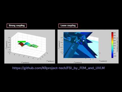
Numerical instability under large fluid density with a loose coupling scheme is caused by added mass term (artificial added mass instability 6). To avoid this problem, the added mass term is included in the structure model 123.

Artificial added mass instability

Proposed fast strong coupling scheme

Comparisons of energy of the sheet between loose coupling and strong coupling FSI analysis
If you use this work in an academic context, please cite the following publication(s):
- Influence of the aspect ratio of the sheet for an electric generator utilizing the rotation of a flapping sheet, Mechanical Engineering Journal, Vol. 8, No. 1 (2021).
https://doi.org/10.1299/mej.20-00459
@article{Akio YAMANO202120-00459,
    title={Influence of the aspect ratio of the sheet for an electric generator utilizing the rotation of a flapping sheet},
    author={Akio YAMANO and Hiroshi IJIMA and Atsuhiko SHINTANI and Chihiro NAKAGAWA and Tomohiro ITO},
    journal={Mechanical Engineering Journal},
    volume={8},
    number={1},
    pages={20-00459-20-00459},
    year={2021},
    doi={10.1299/mej.20-00459}
}
- Flow-induced vibration and energy-harvesting performance analysis for parallelized two flutter-mills considering span-wise plate deformation with geometrical nonlinearity and three-dimensional flow, International Journal of Structural Stability and Dynamics, Vol. 22, No. 14, (2022).
https://doi.org/10.1142/S0219455422501632
@article{doi:10.1142/S0219455422501632,
    author = {Yamano, Akio and Chiba, Masakatsu},
    title = {Flow-Induced Vibration and Energy-Harvesting Performance Analysis for Parallelized Two Flutter-Mills Considering Span-Wise Plate Deformation with Geometrical Nonlinearity and Three-Dimensional Flow},
    journal = {International Journal of Structural Stability and Dynamics},
    volume = {22},
    number = {14},
    pages = {2250163},
    year = {2022},
    doi = {10.1142/S0219455422501632}
}
- Influence of boundary conditions on a flutter-mill, Journal of Sound and Vibration, Vol. 478, No. 21 (2020).
https://doi.org/10.1016/j.jsv.2020.115359
@article{YAMANO2020115359,
    title = {Influence of boundary conditions on a flutter-mill},
    journal = {Journal of Sound and Vibration},
    volume = {478},
    pages = {115359},
    year = {2020},
    doi = {https://doi.org/10.1016/j.jsv.2020.115359},
    author = {A. Yamano and A. Shintani and T. Ito and C. Nakagawa and H. Ijima}
}
├─double_sheets
│  ├─cores
│  │  ├─functions
│  │  │  ├─fluid
│  │  │  └─structure
│  │  └─solver
│  │      ├─fluid
│  │      └─structure
│  ├─save
│  │  └─fig
│  │      └─modes
│  └─ToolBoxes
└─single_sheet
    ├─functions
    │  ├─fluid
    │  └─structure
    ├─save
    │  └─fig
    │      └─modes
    ├─solver
    │  ├─fluid
    │  └─structure
    └─ToolBoxes
[Step 1] Install the ToolBoxes
The following ToolBoxes in “./XXXX/ToolBoxes/” ("XXXX" is "double_sheets" and "single_sheet") are required,
For numerical analysis:
-
“Meshing a plate using four noded elements” by KSSV:
https://jp.mathworks.com/matlabcentral/fileexchange/33731-meshing-a-plate-using-four-noded-elements -
“Sparse sub access” by Bruno Luong:
https://jp.mathworks.com/matlabcentral/fileexchange/23488-sparse-sub-access -
“Vectorized Multi-Dimensional Matrix Multiplication” by Darin Koblick:
https://jp.mathworks.com/matlabcentral/fileexchange/47092-vectorized-multi-dimensional-matrix-multiplication?s_tid=prof_contriblnk
For plotting results:
-
“TriStream” by Matthew Wolinsky:
https://jp.mathworks.com/matlabcentral/fileexchange/11278-tristream -
“mmwrite” by Micah Richert:
https://jp.mathworks.com/matlabcentral/fileexchange/15881-mmwrite -
“Quiver 5” by Bertrand Dano:
https://jp.mathworks.com/matlabcentral/fileexchange/22351-quiver-5?s_tid=FX_rc3_behav
[Step 1.2] Add path to installed ToolBoxes
Modify "add_pathes.m" to add path to abovementined installed ToolBoxes as follows,
addpath ./ToolBoxes/XX;
where XX is the name of folder of the installed ToolBox.
[Step 1.3] Modify the source code in the “TriStream” ToolBox
"TriStream.m" must be modified to plot the stram line Line.
Line 49: x=x(:)'; y=y(:)'; x0=x0(:)'; y0=y0(:)'; u=u(:)'; v=v(:)';
→
x=x(:)'; y=y(:)'; x0=x0(:)'; y0=y0(:)'; u=double(u(:)'); v=double(v(:)');
and
line 63: TRI = tsearch(x,y,tri',Xbeg,Ybeg);
→
TRI = tsearchn([x.' y.'], tri',[Xbeg.' Ybeg.']);
[Step 2] Start GUI form
Open the “GUI.fig” from MATLAB.

[Step 2.1] Pre-setting
Push the "Parameters" buttun and edit parameters.
[Step 3] Start analysis
Push the “exe” button and wait until the finish of the analysis.
[Step 4] Plot results
Push the “plot” button.
[Step 5] View plotted results
Results (figures and movie) plotted by [Step 4] are in "./XXXX/save" directory.
Analytical condisions are in "./XXXX/save/param_setting.m"
%% Analytical conditions
End_Time = 20;                                          %% Nondimensional analysis time [-]
d_t = 1.0e-3;                                           %% Nondimensional step time [-]
core_num = 6;                                           %% Core number [-]
speed_check = 0;                                        %% 1:ON, 0:OFF [-]
alpha_v = 0.5;                                          %% 1:implicit solver,0:explicit solver [-]

Ma = 1.0;                                              %% Mass ratio [-]
Ua = 15.0;                                            	%% Nondimensional flow velocity [-]
theta_a_vec = 0e-1*[ 0 10];                           	%% Nondimensional material damping [-]
-
Mass ratio
$M^*$ is the density ratio of the fluid and sheet, which is defined by,
where
-
Nondimensional flow velocity
$U^*$ represents the free-stream velocity nondimensionalized by the flag rigidity and inertia 123,
where
Initial disturbances on two sheets to break the trivial equilibrium are written as,
q_in_norm = @( time)( 0.5*sin( pi*time/0.2).*( time < 0.2 ) );              %% Initial disturbance (upper sheet)
q_in_norm_1 = @( time)( 0.0*sin( pi*time/0.2).*( time < 0.2 ) );        	%% Initial disturbance (lower sheet)
q_in_vec = [ 0 0 1].';                                                      %% Force direction [-]
Dimensions of sheets are defined by,
Length = 1.0;                                   %% (Nondimensional) length [-]
Width = 1.0;                                    %% aspect ratio [-]
Height = 2.0;                              	    %% distance between two sheets [-]
thick = 1e-3;                                   %% thickness [-]
where the aspect ratio Width is thick is Height is
Boundary conditions for two sheets are written as,
- Clamped at the leading-edge
%% Boundary conditions for two sheets

%%[0] Upper sheet
node_r_0 = [ 1:Ny+1 ];                                                      %% Node number giving the displacement constraint [-]
node_dxr_0 = [ 1:Ny+1 ];                                                    %% Node number giving x-directional gradient constraint [-]
node_dyr_0 = [ 1:Ny+1 ];                                                    %% Node number giving y-directional gradient constraint [-]

%%[1] Lower sheet
node_r_0_1 = [ 1:Ny+1 ];                                                    %% Node number giving the displacement constraint [-]
node_dxr_0_1 = [ 1:Ny+1 ];                                                  %% Node number giving x-directional gradient constraint [-]
node_dyr_0_1 = [ 1:Ny+1 ];                                                  %% Node number giving y-directional gradient constraint [-]
- Pinned at the leading-edge
%% Boundary conditions for two sheets

%%[0] Upper sheet
node_r_0 = [ 1:Ny+1 ];                                                      %% Node number giving the displacement constraint [-]
node_dxr_0 = [ ];                                                           %% Node number giving x-directional gradient constraint [-]
node_dyr_0 = [ 1:Ny+1 ];                                                    %% Node number giving y-directional gradient constraint [-]

%%[1] Lower sheet
node_r_0_1 = [ 1:Ny+1 ];                                                    %% Node number giving the displacement constraint [-]
node_dxr_0_1 = [ ];                                                         %% Node number giving x-directional gradient constraint [-]
node_dyr_0_1 = [ 1:Ny+1 ];                                                  %% Node number giving y-directional gradient constraint [-]
where index in vector shows the node index around a plate element to apply boundary conditions.
 (b) Shell elements on a plate. A flexible sheet is partitioned by shell elements when the number of elements is
 Streamlines around flapping sheets (not streaklines)
 Flow velocity distributions
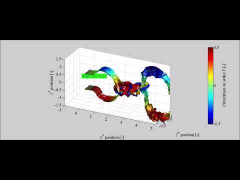
 Wake behind sheets
 Snapshot of two flapping sheets
 Comparisons of snapshot of a flapping sheet under various

MIT License
Issue reports and pull requests are highly welcomed.
Footnotes
-
Influence of the aspect ratio of the sheet for an electric generator utilizing the rotation of a flapping sheet, Mechanical Engineering Journal, Vol. 8, No. 1 (2021).
[OA: https://doi.org/10.1299/mej.20-00459] ↩ ↩2 ↩3 -
Flow-induced vibration and energy-harvesting performance analysis for parallelized two flutter-mills considering span-wise plate deformation with geometrical nonlinearity and three-dimensional flow, International Journal of Structural Stability and Dynamics, Vol. 22, No. 14, (2022).
[https://doi.org/10.1142/S0219455422501632] [OA: https://www.researchgate.net/publication/360386901_Flow-induced_vibration_and_energy-harvesting_performance_analysis_for_parallelized_two_flutter-mills_considering_span-wise_plate_deformation_with_geometrical_nonlinearity_and_three-dimensional_flow] ↩ ↩2 ↩3 ↩4 -
Influence of boundary conditions on a flutter-mill, Journal of Sound and Vibration, Vol. 478, No. 21 (2020).
[https://doi.org/10.1016/j.jsv.2020.115359] ↩ ↩2 ↩3 ↩4 -
J. Katz and A. Plotkin, Low-Speed Aerodynamics, (Cambridge University Press, New York, 2001). ↩
-
A. Shabana, Computational Continuum Mechanics, Chap. 6 (Cambridge University Press, 2008), pp. 231–285. ↩
-
C. Förster, W. A. Wall, E. Ramm, Artificial added mass instabilities in sequential staggered coupling of nonlinear structures and incompressible viscous flows, Computer Methods in Applied Mechanics and Engineering, Vol. 196, No. 7, 2007. ↩
-
M. Chen, L. Jia, Y. Wu, X. Yin, Y. Ma, Bifurcation and chaos of a flag in an inviscid flow, J. Fluid Struct. 45 (2014b) 124-137. ↩