from IPython.display import Image
from IPython.core.display import HTML

The code, weights and logs used for these experiments can be found at 'https://github.com/JakobKallestad/InceptionV3-on-plankton-images'.

Exercise 1 report

By Jakob Kallestad, Eirik Norseng and Eirik Rikstad

Outline:

1. InceptionV3 architecture


2. InceptionV3 algorithm on Cifar10 dataset


3. InceptionV3 algorithm on Plankton dataset

1. InceptionV3 architecture

For this exercise, we have chosen to go with the Inception V3 architecture, trained on the ImageNet dataset. Inception V3 is a CNN, convolutional neural network, a class of networks wich uses the mathematical operaitons pooling and convolutions. In CNNs, this works by applying a filter to the input of any layer. The filter works by doing some operations depending on the filter type and the input. For convolutional filters, the product of filter cells with corresponding cells of the input are added together. For Pooling filters, the maximum, minimum or average value that the filter "covers" are given as output. Under you can see an example of a 2x2 filter from "A guide to convolution arithmetic for deep learning"(Dumoulin & Visin) https://arxiv.org/abs/1603.07285v2.

Image(url= "https://miro.medium.com/max/441/1*BMngs93_rm2_BpJFH2mS0Q.gif")

The filter slides over the input with a predefined step size, called stride, and outputs one number for each position. These filters are usually used more than one at the time. What happens then is that the outputs of each filter is stacked on top of each other, making up the output channels. Each of the individual filter however takes into account all the input channels and adds them together. This gives an output size of OxO, O=(W-K+2P)/S + 1, independent of the number of channels in the input. P in the formula is the padding size. Padding is a technique where one adds "empty" pixels on the edges of the input, to effectively increase the effect of the outmost pixels. In our chosen architecture, the padding is "same", meaning that the padding varies so that the output has the same height and width dimensions as the output.

Inception V3 is as the name suggests a architecture of the Inception type. These are build up of so called Inception module, of which the idea is that instead of chosing a number of filters of one filtersize in a convolutional layer at a point, you chose multiple filter size, and then stack the outputs into one. This allows for detection of objects of different sizes in images in an effective way. The inception module is illustrated in the figure below, from the paper "Going deeper with convolutions"(Szegedy et al., 2014), where the inception network was first introduced. https://arxiv.org/abs/1409.4842

Image(url= "https://miro.medium.com/max/1257/1*DKjGRDd_lJeUfVlY50ojOA.png")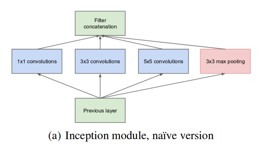

Call this module, the model (a), the naive version. This uses 3 types convolutional filters of size 1x1, 3x3 and 5x5, and a pooling filter. To ensure the output is of the different filters are of the same size, a same padding is used on both the convolutional filter, but also the pooling filter.

This is however an operational costly layer, where the numbers of operations for each convolutional filter is the dimension of the input, height width number of channels, times the dimension of the filter, height width number of filters. To reduce the number of operation, module b is proposed.

Image(url = "https://miro.medium.com/max/1235/1*U_McJnp7Fnif-lw9iIC5Bw.png")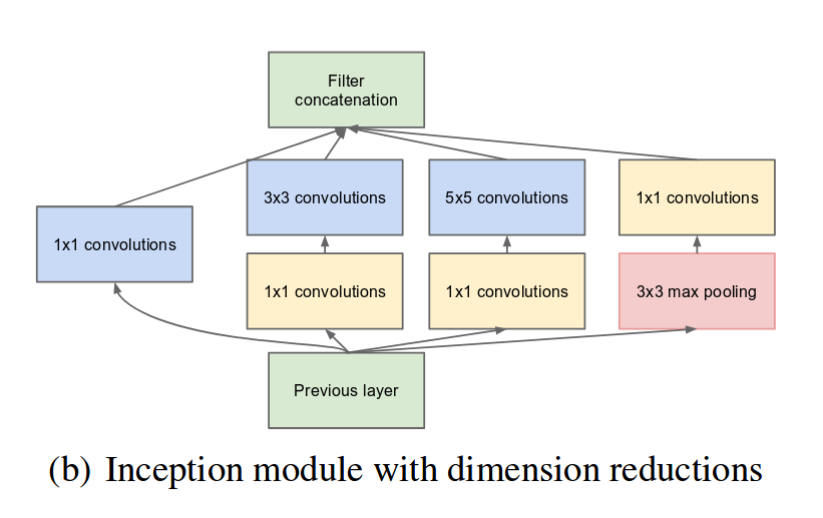

Here the inventors have added a 1x1 filter before the 3x3 and 5x5 filters. Doing this, the dimension of the input are reduced, specifically the number of channels of the input is reduced, and the output of the 1x1 filters, have a number of channels equal to the number of 1x1 filters. Doing this, the cost of going from the input to the output of the 5x5 filters is reduced to the dimension of the input, height width number of channels, times 1x1 times number of 1x1 filters, plus the second filtering, through 5x5, which is equal to the original one in b, divided by the ratio of number of input channels / number of 1x1 filters.

Modules of the b types are used in the inception architecture from the paper, the Inception V1, ending in the architecture in the below figure(source: https://towardsdatascience.com/illustrated-10-cnn-architectures-95d78ace614d#81e0). This is also the baseline for Inception V3, but there are multiple other alterings to the inception modules, which will soon be explained.

Image(url = "https://miro.medium.com/max/2591/1*53uKkbeyzJcdo8PE5TQqqw.png")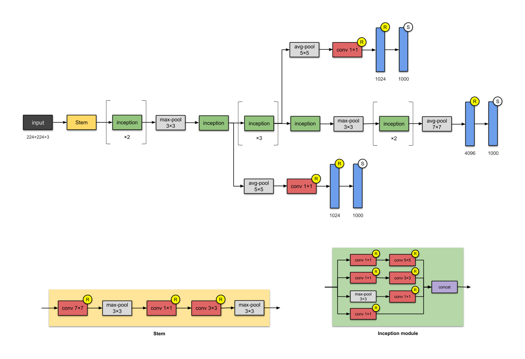

As we can see, the architecture consists of a stem, which consists of traditional pooling and convolutional layer, and then pooling layers in between inception modules. In the end, there is a pooling, a fully connected and a softmax layer.

As mentioned earlier, the Inception V3 as we use, is based on this Inception V1, but with a couple improvements. First of all, 5x5 filters are factorized into two 3x3 filters. As 5x5 filters are more then two times more computionally expensive than 3x3 filters, this decreases number of operations. nxn filters are further factorized into 1xn and nx1 filters, which is reported in the paper to be 33% cheaper than one nxn filter. To avoid the inception modules beeing to deep, the filters are instead spread, to widen the inception modules. The full network are shown in the figure below (source:https://towardsdatascience.com/illustrated-10-cnn-architectures-95d78ace614d#81e0).

Image(url = "https://miro.medium.com/max/3012/1*ooVUXW6BIcoRdsF7kzkMwQ.png")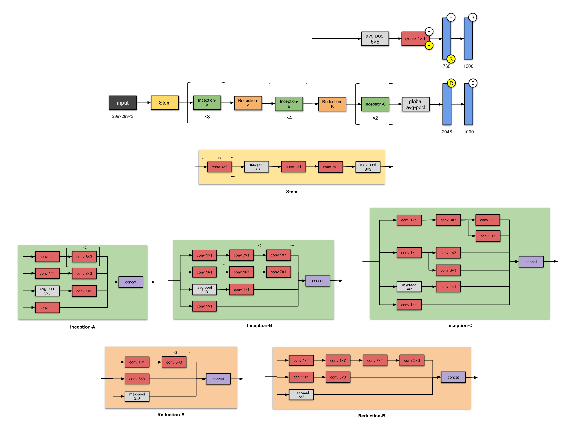

As we can see, the Inception V3 architecture also involves reduction modules, which in principle are the same as inception module, except that it is designed to decrease the dimensions of the input. In total the Inception V3 includes about 24M parameters. It is also worth mentioning that the V3 takes as default input 299x299x3, and uses a RSMProp optimizer. As this is designed for the ImageNet dataset, it outputs 1000 different classes, but as we use it for the plankton dataset, we change the last layers to fit to our desired output.

---

2. InceptionV3 algorithm on Cifar10

Outline:

• The Cifar10 dataset


• Hyperparameters


• Data preprocessing and augmentation


• Training results


• Results on the testset

The Cifar 10 dataset:

The cifar10 dataset is imported from keras, and contains 60 000 images of 10 categories. The number of images per category is evenly distributed with 6000 images from each. All the images are originally RGB images of size (32, 32, 3). We divided this dataset into:

• Train:       40 000 images
• Validation:   10 000 images
• Test:        10 000 images

In order to use less memory and processing time we downloded the dataset and saved it on disk with the code provided in 'create_cifar10data_images.ipynb' file. This code also upscales the images to size (75, 75, 3) because InceptionV3 requires this as a minimum size of training input.

Example images from the dataset after upscaling:

class_names = ['airplane','automobile','bird','cat','deer','dog','frog','horse','ship','truck']

link_list = ['https://raw.githubusercontent.com/JakobKallestad/InceptionV3-on-plankton-images/master/images/cifar10/categories/{}.jpg'.format(cn) for cn in class_names]
html_list = ["<table>"]
html_list.append("<tr>")
for j in range(10):
    html_list.append("<td><center>{}</center><img src='{}'></td>".format(class_names[j], link_list[j]))
html_list.append("</tr>")
html_list.append("</table>")

display(HTML(''.join(html_list)))   

airplane

automobile

bird

cat

deer

dog

frog

horse

ship

truck

Hyper parameters

• optimizer:

  • We used the Adam optimizer because it is very robust and it is forgiving if you specify a non-optimal learning rate.
  • InceptionV3 uses RMSProp as default, but after using RMSProp initially we noticed that we were getting better results with Adam, so ended up using that instead.

• learning rate:

  • 1e-3 (on top layers only)
  • 1e-4 (after unfreezing all layers)

• batch size:

  • We ended up using a batch size of 64
  • That is large enough to ensure a good representation of the 10 classes is each batch, and still not being too computationally heavy.

Data preprocessing and augmentation

• Upscaling:

  • We used the upscale function from cv2 package to enlarge the images.
  • (Instead of just padding the images with zeros)

• ImageDataGenerator:

  • rotation_range=10
  • width_shift_range=0.1
  • height_shift_range=0.1
  • horizontal_flip=True
  • We used these flip and rotational augmentations to decrease the risk of overfitting, and to increase the amount of data that we can train on.
  • shuffle=True
  • Since the training data is organized in order of category, we shuffle the data before every epoch. The model trains on the entire dataset for every epoch.
  • inception's own pre_proccess function. InceptionV3 comes with a pre_process function that normalizes the pixels to values ranging from -1>x<1

Training results

#Accuracy and top_5_accuracy graphs while training of InceptionV3 on Cifar10 dataset:
display(HTML("""<table>                
                <tr>
                <td><center>Accuracy</center><img src='https://raw.githubusercontent.com/JakobKallestad/InceptionV3-on-plankton-images/master/images/cifar10/categorical_accuracy_cifar10_training.png'></td>
                <td><center>Top 5 accuracy</center><img src='https://raw.githubusercontent.com/JakobKallestad/InceptionV3-on-plankton-images/master/images/cifar10/top_5_accuracy_cifar10_training.png'></td>
                </tr>
                </table>"""))

Accuracy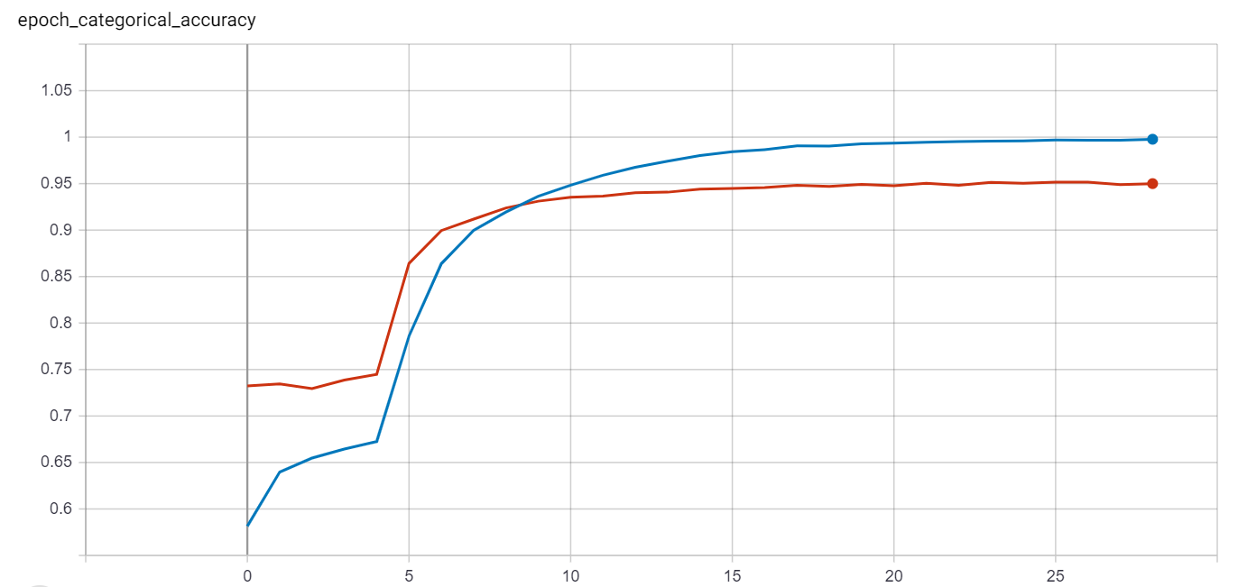

Top 5 accuracy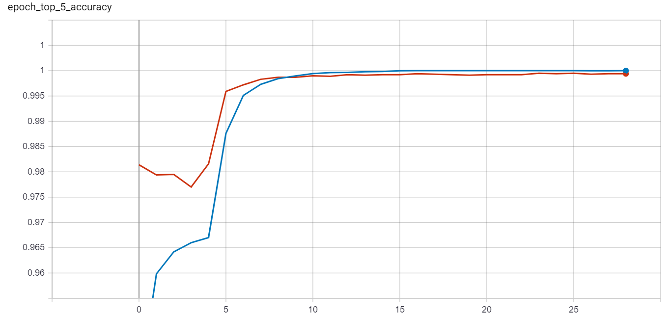

Red = validation data, Blue = training data

The spike of improvement at epoch 4 is because thats when we unfroze all the layers of the network. Not much improvement happened after about epoch 15 for the validation data.

Results after 28 epochs:

• Accuracy:

  • Training data accuracy : 99.77%
  • Validation data accuracy : 95.00%

• Top_5_Accuracy:

  • Validation data accuracy : 99.995%

However, there are only 10 categories, so top 5 accuracy isnt all too interesting.

#Loss for cifar10 training
Image(url= "https://raw.githubusercontent.com/JakobKallestad/InceptionV3-on-plankton-images/master/images/cifar10/loss_cifar10_training.png")

Red = validation data, Blue = training data

The loss function indicates that we might be overfitting the model slightly in the last 10 epochs. However, the loss increase is insignicant and so we stop training and keep the model for testing.

Results on the testset

Image(url= "https://raw.githubusercontent.com/JakobKallestad/InceptionV3-on-plankton-images/master/images/cifar10/accuracy_cifar10_testdata.png")

When evaluating the model on our testset we got an accuracy of 95.42%. Very much what the model predicted on the validation data, indicating that we did not overfit during training. (The results are evaluated with the code in 'running_cifar10_model_on_testset.ipynb.)

#Confusion matrix on test set
Image(url= "https://raw.githubusercontent.com/JakobKallestad/InceptionV3-on-plankton-images/master/images/cifar10/confusion_matrix_cifar10_testdata.png")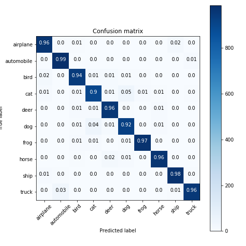

From the confusion matrix we see that categories that most often are mistaken during evaluation are cats and dogs. And they are most likely to be mistaken for eachother. This should come as no surprise as, among these 10 categories, those two are probably the most similar. Even humans can mistake a dog for a cat if the image is of very low resolution. The original images are of size (32, 32).

Possible improvements

After about epoch 15, the model stopped improving on the validation data. To squeeze a better result out of this model we could try to lower the learning rate and increase the amount of augmentation used in the generator.

However, our focus for this exercise was more geared towards the Plankton dataset which demanded most of our virtual machines running time, and so we settled for this result.

---

InceptionV3 algorithm on Plankton dataset

Outline:

• Introduction to the plankton dataset


• Hyperparameters


• Data preprocessing and augmentation


• Initial experiments


• Results

Image(url= "http://33.media.tumblr.com/e8ed810ef98f555994cdcbfd6ec04ab3/tumblr_neot4s0EBL1s2ls31o1_400.gif")

Introduction to plankton dataset:

The plankton dataset that we use contains 712 491 images of plankton spread unevenly accross 65 different species. These are in turn divided into train, validation and test sets with the following ratios:

• Train:       699 491 images
• Validation:   6500 images
• Test:        6500 images

In short we used the train, validate and test folders inside the data-65 folder from the dataset given to us for this assignment.

Here is an overview of what the different species look like:

class_names = ['Acantharea', 'Acartiidae', 'Actinopterygii', 'Annelida', 'Bivalvia__Mollusca', 'Brachyura',
              'bubble', 'Calanidae', 'Calanoida', 'calyptopsis', 'Candaciidae', 'Cavoliniidae', 'Centropagidae',
              'Chaetognatha', 'Copilia', 'Corycaeidae', 'Coscinodiscus', 'Creseidae', 'cyphonaute', 'cypris',
              'Decapoda', 'Doliolida', 'egg__Actinopterygii', 'egg__Cavolinia_inflexa', 'Eucalanidae', 'Euchaetidae',
              'eudoxie__Diphyidae', 'Evadne', 'Foraminifera', 'Fritillariidae', 'gonophore__Diphyidae', 'Haloptilus',
              'Harpacticoida', 'Hyperiidea', 'larvae__Crustacea', 'Limacidae', 'Limacinidae', 'Luciferidae', 'megalopa',
              'multiple__Copepoda', 'nauplii__Cirripedia', 'nauplii__Crustacea', 'nectophore__Diphyidae', 'nectophore__Physonectae', 
              'Neoceratium', 'Noctiluca', 'Obelia', 'Oikopleuridae', 'Oithonidae', 'Oncaeidae', 'Ophiuroidea', 'Ostracoda', 'Penilia',
              'Phaeodaria', 'Podon', 'Pontellidae', 'Rhincalanidae', 'Salpida', 'Sapphirinidae', 'scale', 'seaweed', 'tail__Appendicularia',
              'tail__Chaetognatha', 'Temoridae', 'zoea__Decapoda']
link_list = ['https://raw.githubusercontent.com/JakobKallestad/InceptionV3-on-plankton-images/master/images/plankton/species/{}.jpg'.format(cn) for cn in class_names]
html_list = ["<table>"]
for i in range(8):
    html_list.append("<tr>")
    for j in range(8):
        html_list.append("<td><center>{}</center><img src='{}'></td>".format(class_names[i*8+j], link_list[i*8+j]))
    html_list.append("</tr>")
html_list.append("</table>")

display(HTML(''.join(html_list)))   

Acantharea	Acartiidae	Actinopterygii	Annelida	Bivalvia__Mollusca	Brachyura	bubble	Calanidae
Calanoida	calyptopsis	Candaciidae	Cavoliniidae	Centropagidae	Chaetognatha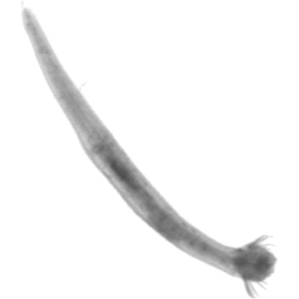	Copilia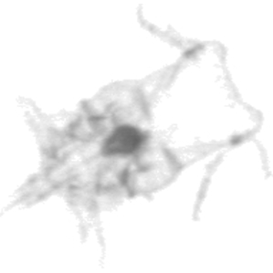	Corycaeidae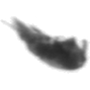
Coscinodiscus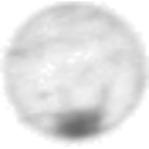	Creseidae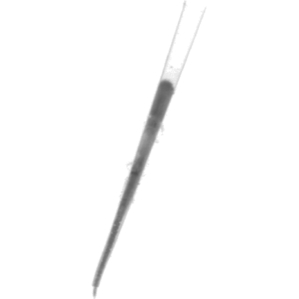	cyphonaute	cypris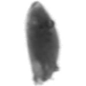	Decapoda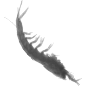	Doliolida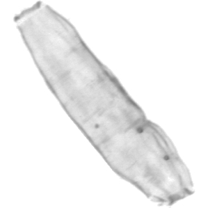	egg__Actinopterygii	egg__Cavolinia_inflexa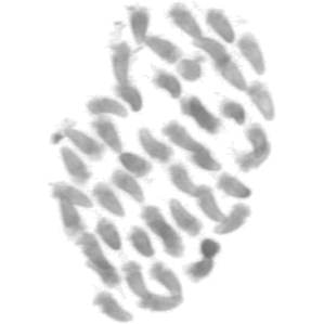
Eucalanidae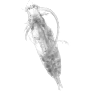	Euchaetidae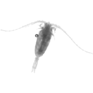	eudoxie__Diphyidae	Evadne	Foraminifera	Fritillariidae	gonophore__Diphyidae	Haloptilus
Harpacticoida	Hyperiidea	larvae__Crustacea	Limacidae	Limacinidae	Luciferidae	megalopa	multiple__Copepoda
nauplii__Cirripedia	nauplii__Crustacea	nectophore__Diphyidae	nectophore__Physonectae	Neoceratium	Noctiluca	Obelia	Oikopleuridae
Oithonidae	Oncaeidae	Ophiuroidea	Ostracoda	Penilia	Phaeodaria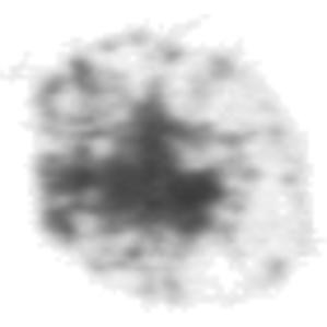	Podon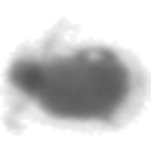	Pontellidae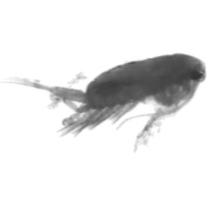
Rhincalanidae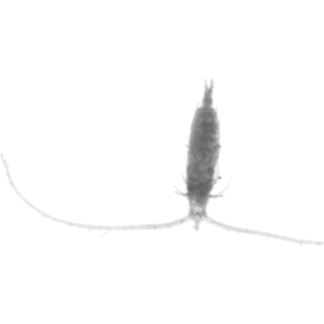	Salpida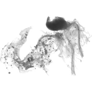	Sapphirinidae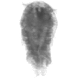	scale	seaweed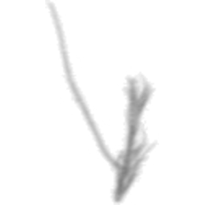	tail__Appendicularia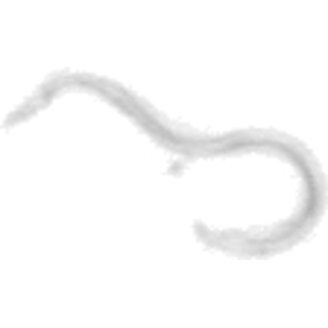	tail__Chaetognatha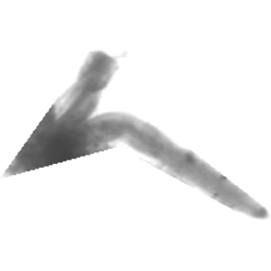	Temoridae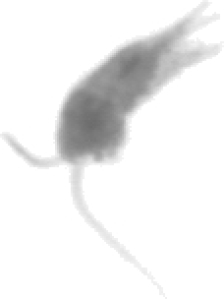

Hyperparameters:

• optimizer:

  • We used the Adam optimizer because it is very robust and it is forgiving if you specify a non-optimal learning rate.
  • InceptionV3 uses RMSProp as default, but after using RMSProp initially we noticed that we were getting better results with Adam, so ended up using that instead.

• learning rate:

  • 1e-3 (on top layers only)
  • 1e-4 (after unfreezing all layers)
  • 1e-5 (for the final few epochs)

• batch size:

  • We used a batch size of 128
  • We wanted a high batch size as there are many classes in the dataset and it is also unbalanced which is not taken into account by the training generator and therefore poses a risk of having very unbalanced batches if they are small.
  • When testing we found that using a batch size of 128 gave significantly better results than a batch size of 64.
  • Due to memory constraint we were not able to test with a higher batch size than 128, but any higher than this might make training too slow anyway.

• steps_per_epoch:

  • train: 1000
  • validate: 51
  • test: 51
  • As there are nearly 700 000 images in the training set and a batch size of 128 this gives us (128*1000)/700000 ≈ 0.2 which means that the model sees about 1/5 of the data per epoch.
  • For test and validation the steps_per_epoch are sufficiently high so that all the data is used to calculate validation and test accuracy/loss.

Data preprocessing and augmentation

• imagedatagenerator:

  • rotation_range=360

  • width_shift_range=0.1

  • height_shift_range=0.1

  • horizontal_flip=True

  • vertical_flip=True

  • inception's own pre_proccess function

  • We used heavy augmentation on the training data. Having the ability to flip and rotate the images freely put us in a situation where we felt that the risk of overfitting was very low.

  • This meant that our main challenge for training a good model was having enough time to train it, and tuning the hyper parameters correctly.

• Datagenerator:

  • shuffle=True

  • The datagenerator shuffles the training data to hopefully create somewhat even batches.

  • Note that it makes sure to go through all the training data before re-shuffeling.

  • target_size=(299, 299)

  • As the plankton dataset contains images of different sizes we used the target_size argument to automatically resize all images to (299, 299) when read from directory.

  • color_mode='rgb'

  • Finally, because the plankton dataset is only grayscale we used the argument color_mode='rgb' to duplicate the channel two times for a total of three equal channels which corresponds to a grayscale image.

• Dealing with class imbalance:

  • we used sklearn.utils.class_weight.compute_class_weight to compute class_weights based on the number of samples per class.
  • We used this as an argument to the models fit method as:
    • class_weight=class_weight
  • This argument means that classes with less samples in are prioritized and therefore has a higher impact on computing the gradient than the classes with more samples.

Initial experiments

Initially we experimented with different settings and hyper parameters and we eventually found out that:

• Adam gave better results than RMSProp
• Often we had set the learning rate too high
• We set too few of the layers to be trainable for a long time
• In addition to this the imagedatagenerator also used a "zoom" augmentation which we eventually decided to drop as the images are cropped quite uniformly in a way that made the zoom potentially harmfull for performance.

Lets take a look at the graph below which shows an overview of the initial experiments:

• In the beginning the model only went over less than 1% of the entire training set per epoch and only the top layers were trainable. This is why there are so many epochs in the graph.

• The first peak was when we decided to unfreeze more layers than just the top layers of inception and made them trainable which increased accuracy from about 8% to about 15%.

• The second peak was when we realized that it helped to increase the batch size and steps_per epoch so that the model over about 20% of the entire training set per epoch.

• The last giant peak happened as soon as we unfroze all the layers of inception for training.

At this point we decided to start from scratch in order to try and recreate the very quick increase in accuracy that the model achieved by the end, but achieve this in less epochs.

# Initial experiments with a maximum of 89% accuracy:
Image(url= "https://raw.githubusercontent.com/JakobKallestad/InceptionV3-on-plankton-images/master/images/plankton/original_acc.png")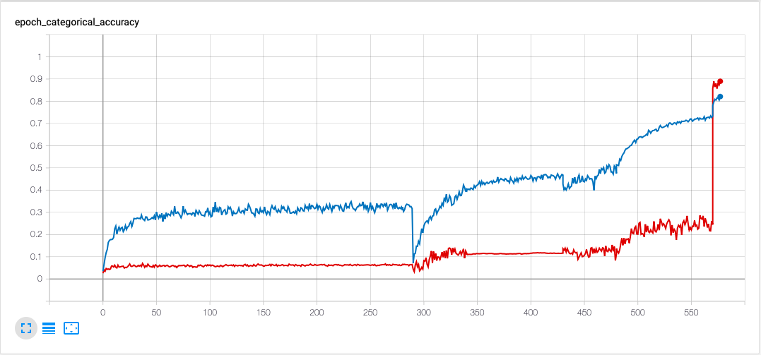

Red = validation data, Blue = training data

New results:

With some intuition learned from our initial experiments we set out to try and replicate the success of how our first model managed to reach 89% accuracy on the validation set, only faster.

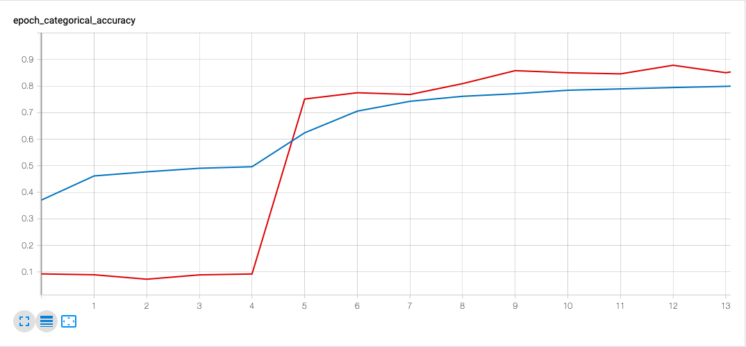
We started of with training only the top layers for 5 epochs and then trained another 10 epochs after that when all the layers were set to be trainable. We left this to run overnight and woke up to great results the next day. The training flattened out in the end with a learning rate of 1e-4, but already at this point it managed to acheive 88% accuracy on the validation set in less than 12 hours of training.

Finally we picked up the training once more and ran the model for 5 more epochs with a learning rate of 1e-5. This time we set steps_per_epoch from 1000 to 5450 so that the model went through all 700 000 images per epochs. The risk of overfitting was still small due to the heavy augmentation from the imagedatagenerator, so this increased the validation accuracy by a few additinal percents to a new best of 92%, our final best.

# Validation accuracy:
Image(url= "https://raw.githubusercontent.com/JakobKallestad/InceptionV3-on-plankton-images/master/images/plankton/new_acc_improved.png")

Red = validation data, Blue = training data

How important was the transfer learning from imagenet?

After we were able to train a good model in less than 12 hours we decided to test how much it mattered that inceptionV3 was pre-trained with weights from imagenet.

We executed the same code again, only this time without loading the weights from imagenet when creating the inceptionV3 model. Then we ran our code overnight for 12 epochs so we could compare the results with and without transfer learning from imagenet.

Our findings show that there was a significant difference between loading the weights from imagenet or leaving the weights to random initialization.

Under is a comparison of the two models:

display(HTML("""<table>                
                <tr>
                <td><center>With imagenet weights</center><img src='https://raw.githubusercontent.com/JakobKallestad/InceptionV3-on-plankton-images/master/images/plankton/new_acc.png'></td>
                <td><center>Without imagenet weights</center><img src='https://raw.githubusercontent.com/JakobKallestad/InceptionV3-on-plankton-images/master/images/plankton/no_transfer_acc.png'></td>
                </tr>
                
                <tr>
                <td><center>With imagenet weights</center><img src='https://raw.githubusercontent.com/JakobKallestad/InceptionV3-on-plankton-images/master/images/plankton/new_cm.gif'></td>
                <td><center>Without imagenet weights</center><img src='https://raw.githubusercontent.com/JakobKallestad/InceptionV3-on-plankton-images/master/images/plankton/no_transfer_cm.gif'></td>
                </tr>
                </table>"""))

With imagenet weights	Without imagenet weights
:-------------------------:	:-------------------------:

Final results on test set:

Image(url= "https://raw.githubusercontent.com/JakobKallestad/InceptionV3-on-plankton-images/master/images/plankton/test_set_scores.png")

The model managed 91.78% accuracy on the test set which is only a 0.5% decrease from what we observed from the validation data during training.

Lets take a look at the confusion matrix below to see how the model performs on all the classes.

Image(url= "https://raw.githubusercontent.com/JakobKallestad/InceptionV3-on-plankton-images/master/images/plankton/final_plankton_cm.png")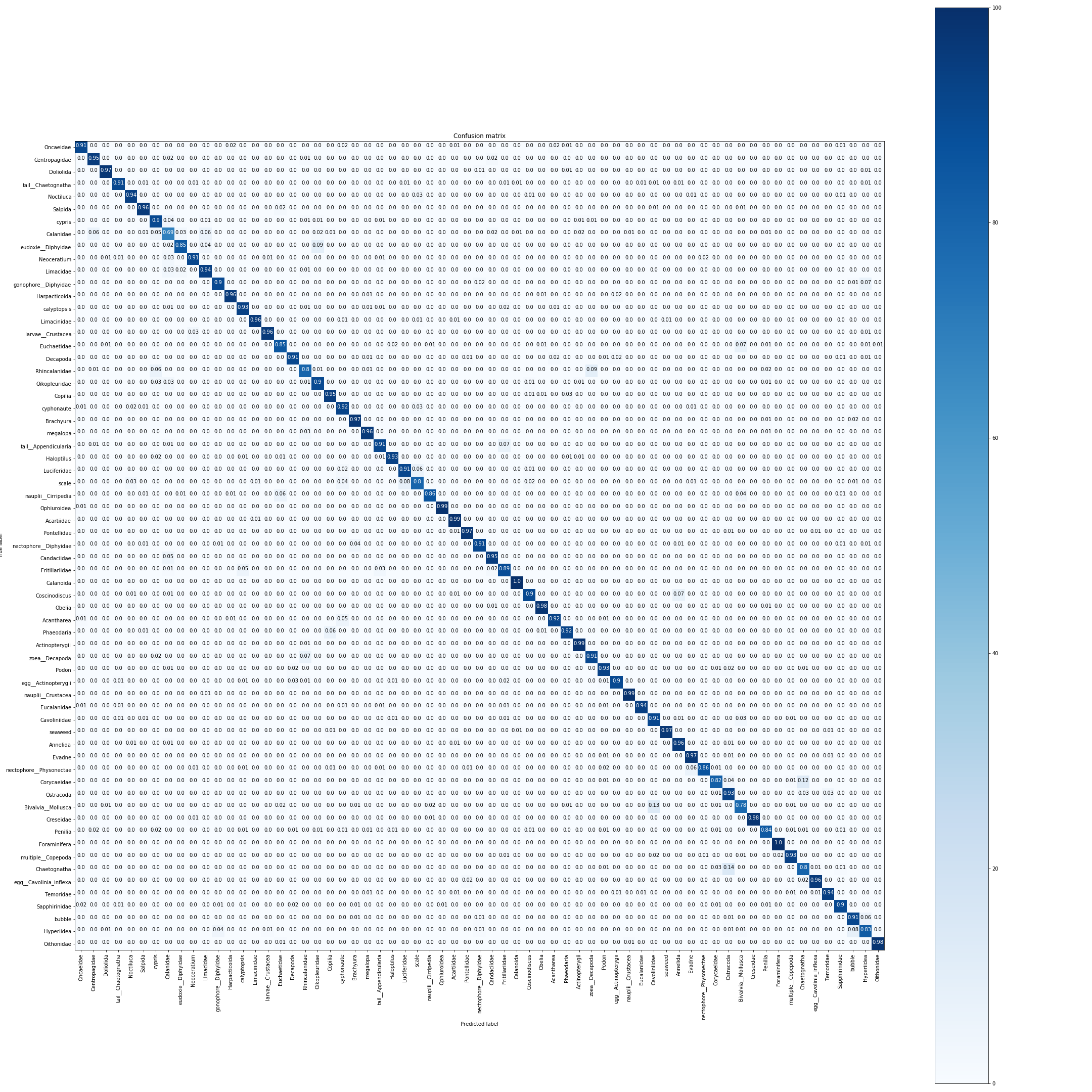

It seems to be quite evenly distributed on all the classes. Taking a closer look at the confusion matrix we see that the model has over 96% accuracy on the top 20 classes, and about 78% accuracy on bottom 5 classes.

The top 2 classes (Calanoida and Foraminifera) has an accuracy of 100% and the worst class (Calanidae) has an accuracy of 69%

---

Tensorboard:

Here are a few magic cells to view our models history via tensorboard interface. The logs folders can be dowloaded from 'https://github.com/JakobKallestad/InceptionV3-on-plankton-images'.

# Run this first:
# !pip install tensorboard
%load_ext tensorboard

Initial Experiments:

%tensorboard --logdir logs5

New version (the best):

%tensorboard --logdir logs6

New version without weights from imagenet:

%tensorboard --logdir logs6_no_transfer