🔥作者🔥忽必烈李@bilibili
注:标数字部分基本内容,未标数字部分为优化内容
[toc]
root是用于粒子物理实验TB或PB及以上数据处理的开源软件,其他特点是数据读取与处理快,并且是一款独立的软件。
ubuntu20.04安装
$ sudo snap install root-framework
$ snap run root-framework
# or if there is no fear of conflicts with other installations:
$ root # and the output of `which root` should contain `/snap`from ROOT import *
h1 =TH1F("h1","Random Numbers",200,-5,5)
h1.FillRandom("gaus")
c1=TCanvas()
h1.Draw()
#input() #显示结果
c1.Print("c1.pdf")
2D直方图
{

    TCanvas *c1 = new TCanvas();
    gStyle->SetPalette(kRainBow); //Palette Style

    TH2F *hist = new TH2F("hist", "Histogram", 100, -1, 1,
                          100, -1, 1);

    hist->SetStats(0);
    TRandom *rand = new TRandom(10);

    for (int i = 0; i < 1e7; i++)

    {
        double x = rand->Gaus();
        double y = rand->Gaus();
        hist->Fill(x, y);
    }


    hist->GetXaxis()->SetTitle("x [cm]");
    hist->GetYaxis()->SetTitle("y [cm]");
    hist->GetZaxis()->SetTitle("Entries");

    hist->Smooth();  //使得图片区域变光滑
    hist->SetContour(1000); //使得palette 变smooth

    hist->Draw("colz"); //colz surf3 cont1 lego2

    c1->Print("colz.png");
}
from __future__ import print_function
from ROOT import TCanvas, TGraph
from ROOT import gROOT
from math import sin
from array import array


c1 = TCanvas( 'c1', 'A Simple Graph Example', 200, 10, 700, 500 )

c1.SetFillColor( 42 )
c1.SetGrid()

n = 20
x, y = array( 'd' ), array( 'd' )

for i in range( n ):
   x.append( 0.1*i )
   y.append( 10*sin( x[i]+0.2 ) )
   print(' i %i %f %f ' % (i,x[i],y[i]))

gr = TGraph( n, x, y )
gr.SetLineColor( 2 )
gr.SetLineWidth( 4 )
gr.SetMarkerColor( 4 )
gr.SetMarkerStyle( 21 )
gr.SetTitle( 'a simple graph' )
gr.GetXaxis().SetTitle( 'X title' )
gr.GetYaxis().SetTitle( 'Y title' )
gr.Draw( 'ACP' )

# TCanvas.Update() draws the frame, after which one can change it
c1.Update()
c1.GetFrame().SetFillColor( 21 )
c1.GetFrame().SetBorderSize( 12 )
c1.Modified()
c1.Update()
# If the graph does not appear, try using the "i" flag, e.g. "python3 -i graph.py"
# This will access the interactive mode after executing the script, and thereby persist
# long enough for the graph to appear.
array 参数的选项

errorbar
from ROOT import TCanvas, TGraphErrors
from ROOT import gROOT
from array import array

c1 = TCanvas( 'c1', 'A Simple Graph with error bars', 200, 10, 700, 500 )

c1.SetGrid()
c1.GetFrame().SetFillColor( 21 )
c1.GetFrame().SetBorderSize( 12 )

n = 10
x  = array( 'f', [ -0.22, 0.05, 0.25, 0.35,  0.5, 0.61,  0.7, 0.85, 0.89, 0.95 ] )
ex = array( 'f', [  0.05,  0.1, 0.07, 0.07, 0.04, 0.05, 0.06, 0.07, 0.08, 0.05 ] )
y  = array( 'f', [     1,  2.9,  5.6,  7.4,  9.0,  9.6,  8.7,  6.3,  4.5,    1 ] )
ey = array( 'f', [  0.8,  0.7,  0.6,  0.5,  0.4,  0.4,  0.5,  0.6,  0.7,  0.8  ] )

gr = TGraphErrors( n, x, y, ex, ey )
gr.SetTitle( 'TGraphErrors Example' )
gr.SetMarkerColor( 4 )
gr.SetMarkerStyle( 21 )
gr.Draw( 'ALP' )

c1.Update()
{
    TCanvas *c1 = new TCanvas();
    TGraphErrors *gr = new TGraphErrors();

    fstream file;
    file.open("data3.txt", ios::in);

    double x, y, ex, ey;
    int n = 0;
    while (1)
    {
        file >> x >> y >> ex >> ey;

        n = gr->GetN();

        gr->SetPoint(n, x, y);
        gr->SetPointError(n, ex, ey);

        if (file.eof())
            break;
    }
    gr->Draw("A*");

    TF1 *fit = new TF1("fit", "pol1", 0, 100);
    gr->Fit("fit");
}
TGraph2D
{
    TCanvas *c = new TCanvas("c", "Graph2D example", 0, 0, 600, 400);
    Double_t x, y, z, P = 6.;
    Int_t np = 200;
    TGraph2D *dt = new TGraph2D();
    dt->SetTitle("Graph title; X axis title; Y axis title; Z axis title");
    TRandom *r = new TRandom();
    for (Int_t N = 0; N < np; N++)
    {
        x = 2 * P * (r->Rndm(N)) - P;
        y = 2 * P * (r->Rndm(N)) - P;
        z = (sin(x) / x) * (sin(y) / y) + 0.2;
        dt->SetPoint(N, x, y, z);
    }
    gStyle->SetPalette(1);
    dt->Draw("colz"); // surf1  CONT5 TRI1 colz

    c->Print("Graph2D.png");

    return c;
}
palette 可选参数
kDeepSea=51,          kGreyScale=52,    kDarkBodyRadiator=53,
kBlueYellow= 54,      kRainBow=55,      kInvertedDarkBodyRadiator=56,
kBird=57,             kCubehelix=58,    kGreenRedViolet=59,
kBlueRedYellow=60,    kOcean=61,        kColorPrintableOnGrey=62,
kAlpine=63,           kAquamarine=64,   kArmy=65,
kAtlantic=66,         kAurora=67,       kAvocado=68,
kBeach=69,            kBlackBody=70,    kBlueGreenYellow=71,
kBrownCyan=72,        kCMYK=73,         kCandy=74,
kCherry=75,           kCoffee=76,       kDarkRainBow=77,
kDarkTerrain=78,      kFall=79,         kFruitPunch=80,
kFuchsia=81,          kGreyYellow=82,   kGreenBrownTerrain=83,
kGreenPink=84,        kIsland=85,       kLake=86,
kLightTemperature=87, kLightTerrain=88, kMint=89,
kNeon=90,             kPastel=91,       kPearl=92,
kPigeon=93,           kPlum=94,         kRedBlue=95,
kRose=96,             kRust=97,         kSandyTerrain=98,
kSienna=99,           kSolar=100,       kSouthWest=101,
kStarryNight=102,     kSunset=103,      kTemperatureMap=104,
kThermometer=105,     kValentine=106,   kVisibleSpectrum=107,
kWaterMelon=108,      kCool=109,        kCopper=110,
kGistEarth=111, kViridis=112, kCividis=113## \file
## \ingroup tutorial_pyroot
## \notebook -js
## This program creates :
## - a one dimensional histogram
## - a two dimensional histogram
## - a profile histogram
## - a memory-resident ntuple
##
## These objects are filled with some random numbers and saved on a file.
##
## \macro_image
## \macro_code
##
## \author Wim Lavrijsen, Enric Tejedor
from ROOT import TCanvas, TFile, TProfile, TNtuple, TH1F, TH2F
from ROOT import gROOT, gBenchmark, gRandom, gSystem
import ctypes
# Create a new canvas, and customize it.
c1 = TCanvas( 'c1', 'Dynamic Filling Example', 200, 10, 700, 500 )
c1.SetFillColor( 42 )
c1.GetFrame().SetFillColor( 21 )
c1.GetFrame().SetBorderSize( 6 )
c1.GetFrame().SetBorderMode( -1 )
# Create a new ROOT binary machine independent file.
# Note that this file may contain any kind of ROOT objects, histograms,
# pictures, graphics objects, detector geometries, tracks, events, etc..
# This file is now becoming the current directory.
hfile = gROOT.FindObject( 'py-hsimple.root' )
if hfile:
hfile.Close()
hfile = TFile( 'py-hsimple.root', 'RECREATE', 'Demo ROOT file with histograms' )
# Create some histograms, a profile histogram and an ntuple
hpx = TH1F( 'hpx', 'This is the px distribution', 100, -4, 4 )
hpxpy = TH2F( 'hpxpy', 'py vs px', 40, -4, 4, 40, -4, 4 )
hprof = TProfile( 'hprof', 'Profile of pz versus px', 100, -4, 4, 0, 20 )
ntuple = TNtuple( 'ntuple', 'Demo ntuple', 'px:py:pz:random:i' )
# Set canvas/frame attributes.
hpx.SetFillColor( 48 )
gBenchmark.Start( 'hsimple' )
# Initialize random number generator.
gRandom.SetSeed()
rannor, rndm = gRandom.Rannor, gRandom.Rndm
# For speed, bind and cache the Fill member functions,
histos = [ 'hpx', 'hpxpy', 'hprof', 'ntuple' ]
for name in histos:
exec('%sFill = %s.Fill' % (name,name))
# Fill histograms randomly.
px_ref, py_ref = ctypes.c_double(), ctypes.c_double()
kUPDATE = 1000
for i in range( 25000 ):
# Generate random values. Use ctypes to pass doubles by reference
rannor( px_ref, py_ref )
# Retrieve the generated values
px = px_ref.value
py = py_ref.value
pz = px*px + py*py
random = rndm(1)
# Fill histograms.
hpx.Fill( px )
hpxpy.Fill( px, py )
hprof.Fill( px, pz )
ntuple.Fill( px, py, pz, random, i )
# Update display every kUPDATE events.
if i and i%kUPDATE == 0:
if i == kUPDATE:
hpx.Draw()
c1.Modified()
c1.Update()
if gSystem.ProcessEvents(): # allow user interrupt
break
# Destroy member functions cache.
for name in histos:
exec('del %sFill' % name)
del histos
gBenchmark.Show( 'hsimple' )
# Save all objects in this file.
hpx.SetFillColor( 0 )
hfile.Write()
hpx.SetFillColor( 48 )
c1.Modified()
c1.Update()
# Note that the file is automatically closed when application terminates
# or when the file destructor is called.## \file
## \ingroup tutorial_pyroot
## \notebook
## Example showing how to fit in a sub-range of an histogram
## An histogram is created and filled with the bin contents and errors
## defined in the table below.
## 3 gaussians are fitted in sub-ranges of this histogram.
## A new function (a sum of 3 gaussians) is fitted on another subrange
## Note that when fitting simple functions, such as gaussians, the initial
## values of parameters are automatically computed by ROOT.
## In the more complicated case of the sum of 3 gaussians, the initial values
## of parameters must be given. In this particular case, the initial values
## are taken from the result of the individual fits.
##
## \macro_output
## \macro_code
##
## \author Wim Lavrijsen
from ROOT import TH1F, TF1
from ROOT import gROOT
from array import array
x = ( 1.913521, 1.953769, 2.347435, 2.883654, 3.493567,
4.047560, 4.337210, 4.364347, 4.563004, 5.054247,
5.194183, 5.380521, 5.303213, 5.384578, 5.563983,
5.728500, 5.685752, 5.080029, 4.251809, 3.372246,
2.207432, 1.227541, 0.8597788,0.8220503,0.8046592,
0.7684097,0.7469761,0.8019787,0.8362375,0.8744895,
0.9143721,0.9462768,0.9285364,0.8954604,0.8410891,
0.7853871,0.7100883,0.6938808,0.7363682,0.7032954,
0.6029015,0.5600163,0.7477068,1.188785, 1.938228,
2.602717, 3.472962, 4.465014, 5.177035 )
np = len(x)
h = TH1F( 'h', 'Example of several fits in subranges', np, 85, 134 )
h.SetMaximum( 7 )
for i in range(np):
h.SetBinContent( i+1, x[i] )
par = array( 'd', 9*[0.] )
g1 = TF1( 'g1', 'gaus', 85, 95 )
g2 = TF1( 'g2', 'gaus', 98, 108 )
g3 = TF1( 'g3', 'gaus', 110, 121 )
total = TF1( 'total', 'gaus(0)+gaus(3)+gaus(6)', 85, 125 )
total.SetLineColor( 2 )
h.Fit( g1, 'R' )
h.Fit( g2, 'R+' )
h.Fit( g3, 'R+' )
par1 = g1.GetParameters()
par2 = g2.GetParameters()
par3 = g3.GetParameters()
par[0], par[1], par[2] = par1[0], par1[1], par1[2]
par[3], par[4], par[5] = par2[0], par2[1], par2[2]
par[6], par[7], par[8] = par3[0], par3[1], par3[2]
total.SetParameters( par )
h.Fit( total, 'R+' )
数据拟合函数参数含义:

{
    TH1F *hist = new TH1F("hist", "Random Numbers", 200, -5, 10);
    hist->FillRandom("gaus");

    hist->SetFillColor(kGreen - 9);

    hist->GetXaxis()->SetTitle("Distribution");
    hist->GetYaxis()->SetTitle("Entries");

    hist->GetXaxis()->SetTitleSize(0.05);
    hist->GetYaxis()->SetTitleSize(0.05);
    hist->GetXaxis()->SetLabelSize(0.05);
    hist->GetYaxis()->SetLabelSize(0.05);

    TF1 *fit = new TF1("fit", "gaus", -5, 5);
    fit->SetLineWidth(3);
    // fit->SetLineColor (kBlue) ;
    fit->SetLineStyle(2);

    fit->SetParameter(0, 40);
    fit->SetParameter(1, 5);
    fit->SetParameter(2, 1);

    TCanvas *c1 = new TCanvas();
    c1->SetTickx();
    c1->SetTicky();
    c1->SetGridx();
    c1->SetGridy();

    //hist
    hist->SetStats(0);
    hist->Draw();
    //fit
    hist->Fit("fit", "R");

    // 图例
    TLegend *leg = new TLegend(0.5, 0.6, 0.8, 0.8);
    leg->SetBorderSize(1);

    leg->AddEntry(hist, "Measured Data", "f");
    leg->AddEntry(fit, "Fit Function", "L");
    leg->Draw();

    double mean = fit->GetParameter(1);
    double sigma = fit->GetParameter(2);
    cout << mean / sigma << endl;

    //添加线条
    TLine *l1 = new TLine(-5,40,10,40);
    l1->SetLineWidth(2);
    l1->SetLineColor(kOrange);
    l1->Draw();

    //添加箭头及文字
    double x0 =1.5;
    int bin = hist->FindBin(x0);
    double y0 = hist->GetBinContent(bin);

    TArrow *arr = new TArrow(4,80,x0,y0);
    arr->SetLineWidth(2);
    arr->SetArrowSize(0.02);
    arr->Draw();

    TLatex *t = new TLatex(4,80,"y=a\\cdot exp(x-\\mu/\\sigma)");
    t->Draw();
}
{
TCanvas *cl = new TCanvas();
TGLViewer *view = (TGLViewer*)gPad->GetViewer3D();
TGeoManager *man = new TGeoManager();
TGeoVolume *top = man->MakeBox("TOP", NULL, 10, 10, 10);
TGeoVolume *box = man->MakeBox("BOX", NULL, 1, 1, 0.2);
box->SetLineColor(kGreen) ;
TGeoHMatrix *trans_rot = new TGeoHMatrix("TRANSROT");
trans_rot->RotateX(45.);
trans_rot->SetDz(2.);
TGeoVolume *tube = man->MakeTube( "TUBE",NULL, 0.5, 1.0, 1.0);
man->SetTopVolume(top) ;

top->AddNode(box, 0);
top->AddNode(box, 1, trans_rot);
top->AddNode(tube,2);

man->CloseGeometry () ;

top->Draw("ogl");

TPolyLine3D *l = new TPolyLine3D();
l->SetLineColor(kRed);
l->SetPoint(0,0,0,0);
l->SetPoint(1,1,1,1);
l->SetPoint(2,0,0,2);
l->Draw("same");
}
结果图

{
    TF1 *f = new TF1("f", "[0]*cos([1]+x)", -5, 5);

    f->SetParameter(0, 1);
    f->SetParameter(1, 1);

    TCanvas *cl = new TCanvas();
    f->Draw();

    ROOT::Math::RootFinder finder;

    finder.Solve(*f, -5, 0);
    double solution = finder.Root();
    cout << solution << endl;

    finder.Solve(*f, 0, 2);
    double solution2 = finder.Root();
    cout << solution2 << endl;

    finder.Solve(*f, 2, 5);
    double solution3 = finder.Root();
    cout << solution3 << endl;

    TLine *l1 = new TLine(-5, 0, 5, 0);
    TLine *l2 = new TLine(solution, -2., solution, 2);
    TLine *l3 = new TLine(solution2, -2., solution2, 2);
    TLine *l4 = new TLine(solution3, -1., solution3, 1);

    l1->Draw();
    l2->Draw();
    l3->Draw();
    l4->Draw();
}
{
    TCanvas *c1 = new TCanvas("c1", "c1", 300, 300);
    TEllipse *el = new TEllipse(0.5, 0.5, 0.1, 0.1);
    el->SetFillColor(kBlack);
    gSystem->Unlink("tut28.gif");

    for (int i = 0; i < 50; i++)
    {
        el->SetX1(0.5 + i * 0.01);
        el->Draw();
        c1->Update();
        c1->Print("tut28.gif+");
        // sleep(1);
    }
}
绘图动画
{
    TCanvas *cl = new TCanvas();

    TH1F *hist = new TH1F("hist", "Histogram", 100, -5, 5);

    gSystem->Unlink("tut29.gif");
    TRandom *r1 = new TRandom();

    for (int i = 0; i < 1e3; i++)
    {
        double val = r1->Gaus();
        hist->Fill(val);
        hist->Draw();
        hist->Fit("gaus");
        cl->Modified();
        cl->Update();
        if (i % 100 == 0)
            cl->Print("tut29.gif+");
        // sleep(1);
    }
}
{
    TVector3 v1(1, 2, 3);

    cout << v1.Y() << endl;
    cout << v1[2] << endl;

    v1.Print();

    double rho = v1.Mag();
    double theta = v1.Theta() * 180. / TMath :: Pi();
    double phi = v1.Phi();

    cout << rho << "\t" << theta << "\t" << phi << endl;
    v1.RotateZ(90 * TMath::Pi() / 180.);
    v1.Print();

    TVector3 v2;

    v2.SetX(4);
    v2.SetY(5);
    v2.SetZ(6);
    v2.Print();

    TVector3 v3;

    v3.SetZ(10);
    v3.SetTheta(10 * TMath ::Pi() / 180.);
    v3.SetPhi(45 * TMath ::Pi() / 180.);
    v3.Print();

    TVector3 v4=v1+v2;
    v4.Print();

    cout<<v1.Dot(v2)<<endl; //向量点乘
    cout<<v1.Angle(v2)*180./TMath::Pi()<<endl; //计算向量夹角

}TClonesArray用于解决频繁的new 与delete占用数据处理时间问题,clonesArray处理重复利用内存问题
void write()
{
    TClonesArray *arr = new TClonesArray("TVector3");
    TClonesArray &ar = *arr;
    TFile *file = new TFile("file.root", "recreate");
    TTree *tree = new TTree("tcl", "tcl");
    tree->Branch("array_branch", &arr);
    TRandom2 *rand = new TRandom2(1);
    for (int i = 0; i < 100; i++)
    {
        /* code */
        arr->Clear();
        for (int j = 0; j < 1000; j++)
        {
            /* code */
            double x = rand->Rndm();
            double y = rand->Rndm();
            double z = rand->Rndm();

            new (ar[j]) TVector3(x, y, z);
        }

        tree->Fill();
    }
    file->Write();
    file->Close();
}

void read()
{
    TFile *file = new TFile("file.root");
    TTree *tree = (TTree*)file->Get("tcl");
    TClonesArray *arr = new TClonesArray("TVector3");
    tree->SetBranchAddress("array_branch",&arr);
    int entries = tree->GetEntries();
    for (int i = 0; i < entries; i++)
    {
        /* code */
        tree->GetEntry(i);
        int lines = arr->GetEntries();
        for (int j = 0; j < lines; j++)
        {
            /* code */
            TVector3 *vec = (TVector3*)arr->At(j);
            cout<<vec->X()<<endl;

        }

    }

}

void tut29()
{
    write();
    read();
}THStack能解决多直方图放到一个途中,y轴不自动变化的问题
{
    THStack *hstack = new THStack("hstack", "Histogram Stack;x title;y title");

    TH1F *hist = new TH1F("hist", "Histogram;x title;y title", 100, -10, 10);
    TH1F *hist2 = new TH1F("hist2", "Histogram 2;x title;y title", 100, -10, 10);

    hstack->Add(hist);
    hstack->Add(hist2);

    hist->FillRandom("gaus", 1e4);
    hist2->FillRandom("gaus", 1e5);

    TCanvas *c2 = new TCanvas();
    c2->Divide(1,2);
    c2->cd(1);
    hist->Draw();
    hist2->Draw("same");
    c2->cd(2);
    hstack->Draw("nostack");

    c2->Print("hstack.png");
}
编写数据处理程序
void processData(TString filename)
{
    TFile *file = new TFile(filename);
}
在终端传入参数给该处理程序
root processData.C("test.root")批量处理ROOT程序,批处理的文件数据格式必须一致。
void write(TString filename)
{
    TFile *output = new TFile(filename, "recreate");
    TTree *tree = new TTree("tree", "tree");
    double x, y;
    tree->Branch("x", &x, "x/D");
    tree->Branch("y", &y, "y/D");

    TRandom2 *r = new TRandom2();
    for (int i = 0; i < 1e6; i++)
    {
        x = 1 + r->Rndm() * 9;
        y = x * 2;
        tree->Fill();
    }
    output->Write();

    output->Close();
}

void chain()
{
    TChain *ch1 = new TChain("tree");  //连接root中的树

    ch1->Add("tuta.root");
    ch1->Add("tutb.root");

    double x;
    ch1->SetBranchAddress("x",&x);

    int entries = ch1->GetEntries();
    TH1F *hist = new TH1F("hist","Histogram",100,1,10);
    for (int i = 0; i < entries; i++)
    {
        /* code */
        ch1->GetEntry(i);
        hist->Fill(x);
    }
    TCanvas *c1 = new TCanvas();
    hist->Draw();
}

void tut29()
{
    write("tuta.root");
    write("tutb.root");

    chain();
}当文件比较大时,可以采用TCut做简单的分析测试
void write(TString filename)
{
    TFile *output = new TFile(filename, "recreate");
    TTree *tree = new TTree("tree", "tree");
    double x, y;
    tree->Branch("x", &x, "x/D");
    tree->Branch("y", &y, "y/D");

    TRandom2 *r = new TRandom2();
    for (int i = 0; i < 1e6; i++)
    {
        x = 1 + r->Rndm() * 9;
        y = x * 2;
        tree->Fill();
    }
    output->Write();

    output->Close();
}

void cut()
{
    TCut cut1 = "x<5";  //设置截断条件
	TCut cut2 = "x>7";
	TFile *input = new TFile("tuta.root","read");
    TTree *tree = (TTree*)input->Get("tree");
	tree->Draw("y",cut1||cut2);
}

void tut29()
{
    write("tuta.root");
    cut();
}
TProfile绘制的直方图与TH1不同,TProfile填充的是Fill(x,y),而TH1只填充Fill(x),y是填充的频率。
TProfile Fill(x,y1)、Fill(x,y2)同一x,不同的y,直方图将采用 $$ (x,\overline y \pm \delta) $$
{
    TCanvas *c1 = new TCanvas();
    TProfile *hprof = new TProfile("hprof", "Profile", 100, 0, 10, "S"); //注意参数S
    TRandom2 *rnd = new TRandom2();
    for (int i = 0; i < 1000; i++)
    {
        hprof->Fill(1, rnd->Rndm());
    }
    hprof->Draw();
}
!!!TProfile能够对多组数据进行直接求方差
#include "TStopwatch.h"
#include "TRandom2.h"
#include "iostream"
using namespace std;

void tut()
{
    TStopwatch t;
    TRandom2 *r = new TRandom2();
    double x=0;
    for(int i=0;i<1e9;i++)
        x +=r->Rndm()
    cout<<x<<endl;
    t.Print();//显示程序运行耗时
}
编译,产生库文件;下次运行能缩短编译时间
root tut.C+ //void transparency()
{
auto c1 = new TCanvas("c1", "c1",224,330,700,527);
c1->Range(-0.125,-0.125,1.125,1.125);
auto tex = new TLatex(0.06303724,0.0194223,"This text is opaque and this line is transparent");
tex->SetLineWidth(2);
tex->Draw();
auto arrow = new TArrow(0.5555158,0.07171314,0.8939828,0.6195219,0.05,"|>");
arrow->SetLineWidth(4);
arrow->SetAngle(30);
arrow->Draw();
// Draw a transparent graph.
Double_t x[10] = {
0.5232808, 0.8724928, 0.9280086, 0.7059456, 0.7399714,
0.4659742, 0.8241404, 0.4838825, 0.7936963, 0.743553};
Double_t y[10] = {
0.7290837, 0.9631474, 0.4775896, 0.6494024, 0.3555777,
0.622012, 0.7938247, 0.9482072, 0.3904382, 0.2410359};
auto graph = new TGraph(10,x,y);
graph->SetLineColorAlpha(46, 0.1);
graph->SetLineWidth(7);
graph->Draw("l");
// Draw an ellipse with opaque colors.
auto ellipse = new TEllipse(0.1740688,0.8352632,0.1518625,0.1010526,0,360,0);
ellipse->SetFillColor(30);
ellipse->SetLineColor(51);
ellipse->SetLineWidth(3);
ellipse->Draw();
// Draw an ellipse with transparent colors, above the previous one.
ellipse = new TEllipse(0.2985315,0.7092105,0.1566977,0.1868421,0,360,0);
ellipse->SetFillColorAlpha(9, 0.571);
ellipse->SetLineColorAlpha(8, 0.464);
ellipse->SetLineWidth(3);
ellipse->Draw();
// Draw a transparent blue text.
tex = new TLatex(0.04871059,0.1837649,"This text is transparent");
tex->SetTextColorAlpha(9, 0.476);
tex->SetTextSize(0.125);
tex->SetTextAngle(26.0);
tex->Draw();
// Draw two transparent markers
auto marker = new TMarker(0.03080229,0.998008,20);
marker->SetMarkerColorAlpha(2, .3);
marker->SetMarkerStyle(20);
marker->SetMarkerSize(1.7);
marker->Draw();
marker = new TMarker(0.1239255,0.8635458,20);
marker->SetMarkerColorAlpha(2, .2);
marker->SetMarkerStyle(20);
marker->SetMarkerSize(1.7);
marker->Draw();
// Draw an opaque marker
marker = new TMarker(0.3047994,0.6344622,20);
marker->SetMarkerColor(2);
marker->SetMarkerStyle(20);
marker->SetMarkerSize(1.7);
marker->Draw();
c1->Print("transparency.pdf");
}窗口显示出错,存为pdf显示正常,采用ghostscript将pdf转换为png
gs -dSAFER -r600 -sDEVICE=pngalpha -o transparency.png transparency.pdf![]()
使用palette的选项卡,PFC (Palette Fill Color), PLC (Palette Line Color) and PMC (Palette Marker Color). When one of these options is given to TH1::Draw the histogram get its color from the current color palette defined by gStyle->SetPalette(...). The color is determined according to the number of objects having palette coloring in the current pad.
/// \file
/// \ingroup tutorial_hist
/// \notebook
/// Palette coloring for histogram is activated thanks to the options `PFC`
/// (Palette Fill Color), `PLC` (Palette Line Color) and `PMC` (Palette Marker Color).
/// When one of these options is given to `TH1::Draw` the histogram get its color
/// from the current color palette defined by `gStyle->SetPalette(...)`. The color
/// is determined according to the number of objects having palette coloring in
/// the current pad.
///
/// In this example five histograms are displayed with palette coloring for lines and
/// and marker. The histograms are drawn with makers and error bars and one can see
/// the color of each histogram is picked inside the default palette `kBird`.
///
/// \macro_image
/// \macro_code
///
/// \author Olivier Couet

void histpalettecolor()
{
   auto C = new TCanvas();

   gStyle->SetOptTitle(kFALSE);
   gStyle->SetOptStat(0);

   auto h1 = new TH1F ("h1","Histogram drawn with full circles",100,-4,4);
   auto h2 = new TH1F ("h2","Histogram drawn with full squares",100,-4,4);
   auto h3 = new TH1F ("h3","Histogram drawn with full triangles up",100,-4,4);
   auto h4 = new TH1F ("h4","Histogram drawn with full triangles down",100,-4,4);
   auto h5 = new TH1F ("h5","Histogram drawn with empty circles",100,-4,4);

   TRandom3 rng;
   Double_t px,py;
   for (Int_t i = 0; i < 25000; i++) {
      rng.Rannor(px,py);
      h1->Fill(px,10.);
      h2->Fill(px, 8.);
      h3->Fill(px, 6.);
      h4->Fill(px, 4.);
      h5->Fill(px, 2.);
   }

   h1->SetMarkerStyle(kFullCircle);
   h2->SetMarkerStyle(kFullSquare);
   h3->SetMarkerStyle(kFullTriangleUp);
   h4->SetMarkerStyle(kFullTriangleDown);
   h5->SetMarkerStyle(kOpenCircle);

   h1->Draw("PLC PMC");  //`PFC` (Palette Fill Color), `PLC` (Palette Line Color) and `PMC` (Palette Marker Color).
   h2->Draw("SAME PLC PMC");
   h3->Draw("SAME PLC PMC");
   h4->Draw("SAME PLC PMC");
   h5->Draw("SAME PLC PMC");

   gPad->BuildLegend();
}

下载root 源文件,解压获得tutorial文件。分别采用python和c++运行root 的demo, 点开Browser查看案例演示及源代码。

方法1:
进入tutorial中的pyroot文件夹,运行
pyroot demo.py方法2:
进入tutorial文件夹,运行
root demos.C1.rootlogon.C
文件路径:$ROOTSYS/tutorials/rootlogon.C
rootlogon.C文件在root启动的当前目录下会被自动调用执行,进行满足用户的特殊配置要求。例如,导入自己的库,设置自己绘图样式
a. 导入自己编译的库
想要导入自己的库函数,在rootlogon.C文件内可加入
gSystem->Load("xxx.so")b. 设置自己的绘图样式
// This is the file rootlogon.c
{
TStyle *mystyle = new TStyle("MyStyle","My Root Styles");

// from ROOT plain style
myStyle->SetCanvasBorderMode (0) ;
myStyle->SetPadBorderMode (0) ;
myStyle—>SetPadcolor (0) ;
myStyle->SetCanvasColor (0) ;
myStyle->SetTitleColor (1) ;
myStyle->SetStatcolor (0) ;
myStyle->SetLabelSize(0.03,"xyz"); // size of axis values

// default canvas positioning
myStyle->setCanvasDefX (900) ;
myStyle—>SetCanvasDefY (20) ;
myStyle->setCanvasDefH (550) ;
myStyle->setCanvasDefW(540) ;

myStyle->SetPadBottomMargin (0.1) ;
myStyle->SetPadTopMargin (0.1) ;
myStyle—>setPadLeftMargin (0.1) ;
myStyle—>SetPadRightMargin (0.1) ;
myStyle->SetPadTickX (1);
myStyle—>SetPadTickY (1) ;
myStyle—>SetFrameBorderMode (0) ;

// Din letter
myStyle->SetPaperSize(21, 28);//show overflow and underflow
myStyle->SetOptStat(111111);
myStyle->SetOptFit(1011);
myStyle->SetPalette(1);

//apply the new style
gROOT->SetStyle("MyStyle"); //uncomment to set this style
gROOT->ForceStyle(); //use this style,not the one saved in root files
printf("\n Beginning new ROOT session with private TStyle \n");

}
2. 将常用代码放到一个文件中以提高效率
将常用文件放到一个文件中,如useful.h

useful.h文件:
#include <TStyle.h>
// Set the general style options
void SetSgStyle()
{
    // No Canvas Border
    gStyle->SetCanvasBorderMode(0);
    gStyle->SetCanvasBorderSize(0);
    // White BG
    gStyle->SetCanvasColor(10);
    // Format for axes
    gStyle->SetLabelFont(22, "xyz");
    gStyle->SetLabelSize(0.06, "xyz");
    gStyle->SetLabelOffset(0.01, "xyz");
    gStyle->SetNdivisions(510, "xyz");
    gStyle->SetTitleFont(22, "xyz");
    gStyle->SetTitleColor(1, "xyz");
    gStyle->SetTitleSize(0.06, "xyz");
    gStyle->SetTitleOffset(0.91);
    gStyle->SetTitleYOffset(1.1);
    // No pad borders
    gStyle-> SetPadBorderMode(0);
    gStyle->SetPadBorderSize(0);
    // White BG
    gStyle->SetPadColor(10);
    // Margins for labels etc.
    gStyle->SetPadLeftMargin(0.15);
    gStyle->SetPadBottomMargin(0.15);
    gStyle->SetPadRightMargin(0.05);
    gStyle->SetPadTopMargin(0.06);
    // No error bars in x direction
    gStyle->SetErrorX(0);
    // Format legend
    gStyle->SetLegendBorderSize(0);
    gStyle->SetFillStyle(0);
}在useful.h中加入:
// 设置Latex放置位置(x0,y0),直方图,字符串,字体大小
void txtN(Double_t x0, Double_t y0, TH1 *h, Char_t sName[] = "N=%.0f", Double_t sizeTxt = 0.06)
{
    h->SetStats(kFALSE);
    TLatex *ltx = new TLatex();
    ltx->SetNDC(kTRUE);
    ltx->SetTextColor(h->GetLineColor());
    ltx->SetTextFont(22);
    ltx->SetTextSize(sizeTxt);
    ltx->DrawLatex(x0, y0, Form(sName, h->GetEntries()));
    gPad->Modified();
    gPad->Update();
}testStyle.C文件:
#include "useful.h"
void testStyle()
{
    TH1F *h1 = new TH1F("h1","",100,-10,10);
    SetSgStyle();
    TH1F *h2 = new TH1F("h2","",100,-10,10);
    h1->FillRandom("gaus",1000);
    h2->FillRandom("gaus",1000);
    TCanvas *c1 = new TCanvas("c1","");
    c1->Divide(2,1);
    c1->cd(1);
    h1->Draw();
    c1->cd(2);
    h2->Draw();
    txtN(0.2,0.95,h2);// 自定义格式
}
在useful.h中加入:
// hist名称,bin宽度,bin上下限,设置MeV标题,设置Mark样式
TH1F * newTH1F(Char_t name[]="h1",Double_t binw=0.01, Double_t LowBin=0.0,Double_t HighBin=3.0,Bool_t MevTitle=kTRUE,Int_t iMode=-1)
{
    Int_t nbin = TMath::Nint((HighBin-LowBin)/binw);
    HighBin = binw*nbin + LowBin;

    TH1F *h = new TH1F(name,"",nbin,LowBin,HighBin);
    if(MevTitle)
        h->GetYaxis->SetTitle(Form("Events/(%.0fMeV/c^{2})",h->GetBinWidth(1)*1000));
    h->SetMinimum(0.0);
    h->GetYaxis()->SetTitleOffset(1.1);
    if(iMode>=0&&iMode<14){
        Int_t iMarker[] ={20,21,24,25,28,29,30,27,3,5,2,,26,22,23};
        Int_t iColor[]={2,4,6,9,1,50,40,31,41,35,44,38,47,12};
        h->SetMarkerStyle(iMarker[iMode]);
        h->SetMarkerColor(iColor[iMode]);
        h->SetLineColor(iColor[iMode]);
    }
    return h;
}
// LineX1: 线的位置,颜色,宽度
void LineX1(Double_t atX, Int_t iColor=kRed, Int_t iStyle=1,Double_t iWidth=1)
{
    gPad->Modified();
    gPad->Update();
    TLine *l1 = new TLine(atX,gPad->GetUymin(),gPad->GetUymax());
    l1->SetLineColor(iColor);
    l1->SetLineStyle(iStyle);
    l1->SetLineWidth(iWidth);
    l1->Draw();
}使用案例,testStyle2
#include "useful.h"
void testStyle2()
{
    TH1F *h1 = newTH1F("h1",0.5,-10,10,kTRUE,1);
    SetSgStyle();
    TH1F *h2 = newTH1F("h2",0.5,-10,10,kTRUE,2);
    h1->FillRandom("gaus",1000);
    h2->FillRandom("gaus",1000);
    TCanvas *c1 = new TCanvas("c1","");
    c1->Divide(2,1);
    c1->cd(1);
    h1->Draw("EP");
    c1->cd(2);
    h2->Draw("EP");
    txtN(0.2,0.95,h2);
    LineX1(0.0);
}
王思广老师的模板:CommonCUtsPureROOT.h
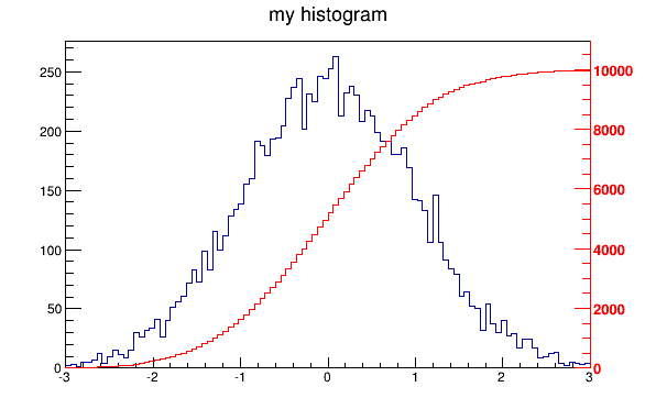
以下脚本创建两个直方图;第二直方图是第一直方图的bins积分。它显示了在同一个Pad中绘制两个直方图的过程,并使用右侧的新垂直轴绘制第二个直方图横坐标。
void twoscales() {
   TCanvas *c1 = new TCanvas("c1","different scales hists",600,400);
   //create, fill and draw h1
   gStyle->SetOptStat(kFALSE);
   TH1F *h1 = new TH1F("h1","my histogram",100,-3,3);
   for (Int_t i=0;i<10000;i++) h1->Fill(gRandom->Gaus(0,1));
   h1->Draw();
   c1->Update();
   //create hint1 filled with the bins integral of h1
   TH1F *hint1 = new TH1F("hint1","h1 bins integral",100,-3,3);
   Float_t sum = 0;
   for (Int_t i=1;i<=100;i++) {
      sum += h1->GetBinContent(i);
      hint1->SetBinContent(i,sum);
   }
   //scale hint1 to the pad coordinates
   Float_t rightmax = 1.1*hint1->GetMaximum();
   Float_t scale    = gPad->GetUymax()/rightmax;
   hint1->SetLineColor(kRed);
   hint1->Scale(scale);
   hint1->Draw("same");
   //draw an axis on the right side
   TGaxis*axis = new TGaxis(gPad->GetUxmax(),gPad->GetUymin(),
                            gPad->GetUxmax(),gPad->GetUymax(),
                            0,rightmax,510,"+L");
   axis->SetLineColor(kRed);
   axis->SetLabelColor(kRed);
   axis->Draw();
}
-
SetBranchAddress (推荐) 能用于读取string类型的数据,可读任意branch,定义步骤较多
-
TTreeReaderValue 定义步骤少,较方便,但只能逐个读取,读取tree中所有的值
//====================TreeReader=============================
	TFile *f = new TFile("output.root");
    TTreeReader fReader("Det", f);
    TTreeReaderArray<Char_t> SDName = {fReader, "SDName"};
    TTreeReaderArray<Char_t> PName = {fReader, "PName"};

    while (fReader.Next())
    {
        //处理数据
    }

//=====================SetBranchAddress=======================
    TFile *f = new TFile("output1.root");
    TTree *t = (TTree *)f->Get("Det");
    Char_t SDName[32],PName[32];

    t->SetBranchAddress("SDName",SDName);
    t->SetBranchAddress("PName",PName);

    Long64_t nEntries = t->GetEntries("PName");
    for (Long64_t i = 0; i < nEntries; i++)
    {
        std::cout<<"PName :"<<PName<<std::endl;
    }
参考资料:
[1] 华文慕课 王思广 root数据分析 http://www.chinesemooc.org/course.php?ac=course_view&id=1083822&eid=69749
[2] root官网使用手册 https://root.cern/root/htmldoc/guides/users-guide/ROOTUsersGuide.html
[3] 法国物理学家 youtube教程 https://www.youtube.com/playlist?list=PLLybgCU6QCGWLdDO4ZDaB0kLrO3maeYAe