100 Core Tree Data Structure Interview Questions

You can also find all 100 answers here 👉 Devinterview.io - Tree Data Structure

1. What is a Tree Data Structure?

A tree data structure is a hierarchical collection of nodes, typically visualized with a root at the top. Trees are typically used for representing relationships, hierarchies, and facilitating efficient data operations.

Core Definitions

• Node: The basic unit of a tree that contains data and may link to child nodes.
• Root: The tree's topmost node; no nodes point to the root.
• Parent / Child: Nodes with a direct connection; a parent points to its children.
• Leaf: A node that has no children.
• Edge: A link or reference from one node to another.
• Depth: The level of a node, or its distance from the root.
• Height: Maximum depth of any node in the tree.

Key Characteristics

• Hierarchical: Organized in parent-child relationships.
• Non-Sequential: Non-linear data storage ensures flexible and efficient access patterns.
• Directed: Nodes are connected unidirectionally.
• Acyclic: Trees do not have loops or cycles.
• Diverse Node Roles: Such as root and leaf.

Visual Representation

Common Tree Variants

• Binary Tree: Each node has a maximum of two children.
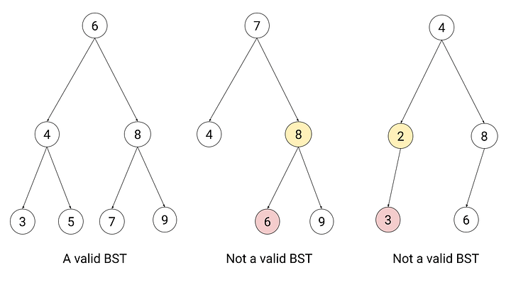
• Binary Search Tree (BST): A binary tree where each node's left subtree has values less than the node and the right subtree has values greater.
• AVL Tree: A BST that self-balances to optimize searches.
• B-Tree: Commonly used in databases to enable efficient access.
• Red-Black Tree: A BST that maintains balance using node coloring.
• Trie: Specifically designed for efficient string operations.

Practical Applications

• File Systems: Model directories and files.
• AI and Decision Making: Decision trees help in evaluating possible actions.
• Database Systems: Many databases use trees to index data efficiently.

Tree Traversals

Depth-First Search

• Preorder: Root, Left, Right.
• Inorder: Left, Root, Right (specific to binary trees).
• Postorder: Left, Right, Root.

Breadth-First Search

• Level Order: Traverse nodes by depth, moving from left to right.

Code Example: Binary Tree

Here is the Python code:

class Node:
    def __init__(self, data):
        self.left = None
        self.right = None
        self.data = data

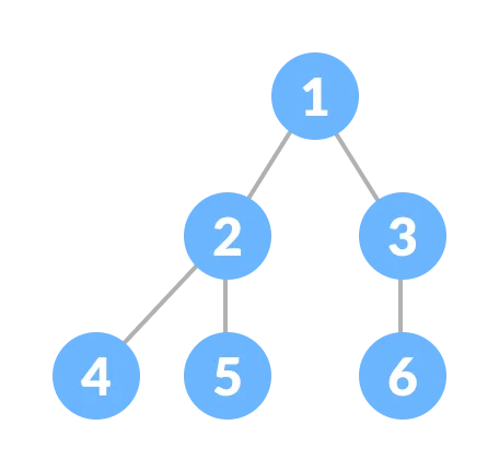
# Create a tree structure
root = Node(1)
root.left, root.right = Node(2), Node(3)
root.left.left, root.right.right = Node(4), Node(5)

# Inorder traversal
def inorder_traversal(node):
    if node:
        inorder_traversal(node.left)
        print(node.data, end=' ')
        inorder_traversal(node.right)

# Expected Output: 4 2 1 3 5
print("Inorder Traversal: ")
inorder_traversal(root)

2. What is a Binary Tree?

A Binary Tree is a hierarchical structure where each node has up to two children, termed as left child and right child. Each node holds a data element and pointers to its left and right children.

Binary Tree Types

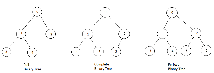
• Full Binary Tree: Nodes either have two children or none.
• Complete Binary Tree: Every level, except possibly the last, is completely filled, with nodes skewed to the left.
• Perfect Binary Tree: All internal nodes have two children, and leaves exist on the same level.

Visual Representation

Applications

• Binary Search Trees: Efficient in lookup, addition, and removal operations.
• Expression Trees: Evaluate mathematical expressions.
• Heap: Backbone of priority queues.
• Trie: Optimized for string searches.

Code Example: Binary Tree & In-order Traversal

Here is the Python code:

class Node:
    """Binary tree node with left and right child."""
    def __init__(self, data):
        self.left = None
        self.right = None
        self.data = data

    def insert(self, data):
        """Inserts a node into the tree."""
        if data < self.data:
            if self.left is None:
                self.left = Node(data)
            else:
                self.left.insert(data)
        elif data > self.data:
            if self.right is None:
                self.right = Node(data)
            else:
                self.right.insert(data)

    def in_order_traversal(self):
        """Performs in-order traversal and returns a list of nodes."""
        nodes = []
        if self.left:
            nodes += self.left.in_order_traversal()
        nodes.append(self.data)
        if self.right:
            nodes += self.right.in_order_traversal()
        return nodes


# Example usage:
# 1. Instantiate the root of the tree
root = Node(50)

# 2. Insert nodes (This will implicitly form a Binary Search Tree for simplicity)
values_to_insert = [30, 70, 20, 40, 60, 80]
for val in values_to_insert:
    root.insert(val)

# 3. Perform in-order traversal
print(root.in_order_traversal())  # Expected Output: [20, 30, 40, 50, 60, 70, 80]

3. Explain Height and Depths in the context of a Tree.

In tree data structures, the terms height and depth refer to different attributes of nodes.

Height

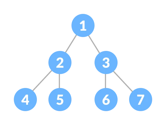
The height of a node is the number of edges on the longest downward path between that node and a leaf.

• Height of a Node: Number of edges in the longest path from that node to any leaf.
• Height of a Tree: Essentially the height of its root node.

Depth

The depth or level of a node represents the number of edges on the path from the root node to that node.

For instance, in a binary tree, if a node is at depth 2, it means there are two edges between the root and that node.

Visual Representation

Code Example: Calculating Height and Depth

Here is the Python code:

class Node:
    def __init__(self, data, parent=None):
        self.data = data
        self.left = None
        self.right = None
        self.parent = parent

def height(node):
    if node is None:
        return -1
    left_height = height(node.left)
    right_height = height(node.right)
    return 1 + max(left_height, right_height)

def depth(node, root):
    if node is None:
        return -1
    dist = 0
    while node != root:
        dist += 1
        node = node.parent
    return dist

# Create a sample tree
root = Node(1)
root.left = Node(2, root)
root.right = Node(3, root)
root.left.left = Node(4, root.left)
root.left.right = Node(5, root.left)

# Test height and depth functions
print("Height of tree:", height(root))
print("Depth of node 4:", depth(root.left.left, root))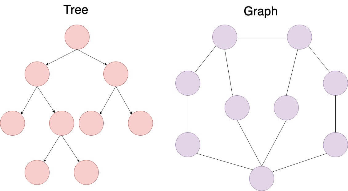
print("Depth of node 5:", depth(root.left.right, root))

4. What is the difference between a Tree and a Graph?

Graphs and trees are both nonlinear data structures, but there are fundamental distinctions between them.

Key Distinctions

• Uniqueness: Trees have a single root, while graphs may not have such a concept.
• Topology: Trees are hierarchical, while graphs can exhibit various structures.
• Focus: Graphs center on relationships between individual nodes, whereas trees emphasize the relationship between nodes and a common root.

Graphs: Versatile and Unstructured

• Elements: Composed of vertices/nodes (denoted as V) and edges (E) representing relationships. Multiple edges and loops are possible.
• Directionality: Edges can be directed or undirected.
• Connectivity: May be disconnected, with sets of vertices that aren't reachable from others.
• Loops: Can contain cycles.

Trees: Hierarchical and Organized

• Elements: Consist of nodes with parent-child relationships.
• Directionality: Edges are strictly parent-to-child.
• Connectivity: Every node is accessible from the unique root node.
• Loops: Cycles are not allowed.

Visual Representation

5. Define Leaf and Internal nodes in a Tree.

In the context of a tree data structure, nodes can take on distinct roles:

Leaf Nodes

• Definition: Nodes without children are leaf nodes. They are the tree endpoints.
• Properties:
  • In a binary tree, leaf nodes have either one or no leaves.
  • They're the only nodes with a depth.
• Visual Representation:
  • In a traditional tree visualization, leaf nodes are the ones at the "bottom" of the tree.

Internal Nodes

• Definition: Internal nodes, or non-leaf nodes, have at least one child.
• Properties:
  • They have at least one child.
  • They're "in-between" nodes that connect other nodes in the tree.
• Visual Representation:
  • In a tree diagram, any node that is not a leaf node is an internal node.
  • The root, which is often at the "top" in visual representations, is also an internal node.

6. What is a Rooted Tree, and how does it differ from an Unrooted Tree?

In computer science, a rooted tree — often referred to as just a "tree" — is a data structure that consists of nodes connected by edges, typically in a top-down orientation.

Each tree has exactly one root node, from which all other nodes are reachable. Rooted trees are distinct from unrooted trees, as the latter does not have a designated starting point.

Key Concepts

• Root Node: The unique starting node of the tree.
• Parent and Children: Nodes are arranged in a hierarchical manner. The root is the parent of all other nodes, and each node can have multiple children but only one parent.
• Leaf Nodes: Nodes that have no children.
• Depth: The length of the path from a node to the root. The root has a depth of 0.
• Height: The length of the longest path from a node to a leaf.

Visual Comparison

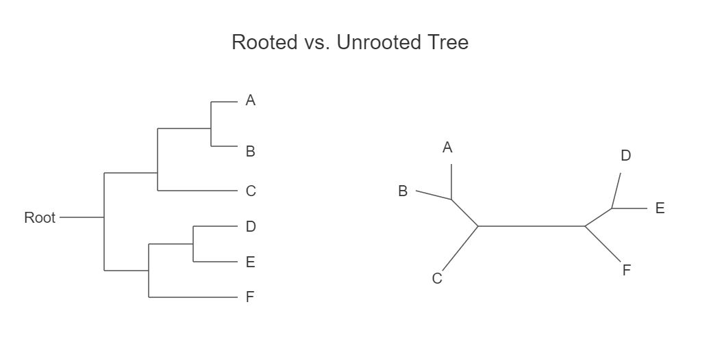
The left side represents a rooted tree with a clear root node. The right side features an unrooted tree, where no such distinction exists.

Code Example: Rooted Tree

Here is the Python code:

class Node:
    def __init__(self, data):
        self.data = data
        self.children = []

# Example of a rooted tree
root = Node('A')
child1 = Node('B')
child2 = Node('C')

root.children.append(child1)
root.children.append(child2)

child3 = Node('D')
child1.children.append(child3)

# Output: A -> B -> D and A -> C

Code Example: Unrooted Tree

Here is the Python code:

class Node:
    def __init__(self, data):
        self.data = data
        self.neighbours = set()

# Example of an unrooted tree
node1 = Node('A')
node2 = Node('B')
node3 = Node('C')

# Connections
node1.neighbours |= {node2, node3}
node2.neighbours.add(node3)

# Output: A <-> B, A <-> C, B <-> C

Practical Applications

• File Systems: Representing directory structures where each directory is a node of a rooted tree.
• HTML DOM: Visualized as a tree with the HTML tag being the root.

Unrooted Trees in Nature

• Phylogenetic Trees: Used to represent the evolutionary relationships among a group of species without a clear ancestor.
• Stemmatology: In textual criticism, they're used to describe textual relationships without identifying an original or "root" text.

7. What is a N-ary Tree, and how does it generalize a binary tree?

An N-ary Tree is a data structure with nodes that can have up to $N$ children, allowing for more than two child nodes. This property provides the tree with a more flexible hierarchical structure compared to the strict two-child policy observed in binary trees, permitting either a binary or non-binary organization of nodes, as per the figure below.

N-ary Tree Representation

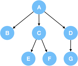
In N-ary Trees, nodes can have a dynamic number of child nodes, dictated by the length of a list or array where these nodes are stored. This contrasts with the binary tree, where nodes have a fixed, often predefined, number of children (either 0, 1, or 2).

Some embodiments conveniently use an array, where each element corresponds to a child. While this allows for $O(1)$ child lookups, a la binary heap. It does mean that every internal node has N slots, wasting memory on nodes with fewer children.

Code Example: N-ary Tree Node

Here is the Python code:

class Node:
    def __init__(self, data, children=None):
        self.data = data
        self.children = children if children else []

    def add_child(self, child):
        self.children.append(child)

Use of N-ary Trees

1. File Systems: Represent directories and files, where a directory can have multiple subdirectories or files.

2. Abstract Syntax Trees (ASTs): Used in programming languages to represent the structure of source code. A node in the AST can correspond to various constructs in the code, such as an expression, statement, or declaration.

3. Multi-way Trees: Employed in the management of organized data, particularly in the index structures of databases or data warehouses.

4. User Interfaces: Structures with multiple child components, like list views, trees, or tabbed panels, exemplify the role of n-ary trees in this domain.

5. Data Analytics and Machine Learning: Classification and decision-making processes often entail using multi-way trees, such as N-ary decision trees.

8. Discuss the properties of a Full Binary Tree.

A Full Binary Tree, often referred to as a "strictly binary tree," is a rich mathematical structure that presents a distinctive set of characteristics.

It is a tree data structure in which each node has either zero or two children. Every leaf node is found at the same level, and the tree is perfectly balanced, reaching its most compact organizational form.

Full Binary Tree Properties

Node Count

• The number of nodes in a Full Binary Tree, $N$, is odd for a finite tree due to the one-root node.
• With $N+1$ nodes, a Full Binary Tree may still be complete (not full).
• The $n$th level holds between $\frac{n}{2}+1$ and $n$ nodes, with all levels either full or skipping just the last node.

Relationship between Node Count and Tree Height

• A Full Binary Tree's height, $h$, can range from $\log_2(N+1) - 1$ (for balanced trees) to $N - 1$ (for degenerate trees).

External Nodes (Leaves)

• The number of leaves, $L$, is:
  • even when $N$ is one less than a power of two.
  • odd when $N$ is equal to a power of two.
• A Full Binary Tree always has one more non-leaf node than leaf nodes.

Parent-Child Relationship

• The parent of the $n$th node in a Full Binary Tree is given by:

  $$ \text{parent}(n) = \Bigg \lceil \frac{n}{2} \Bigg \rceil - 1 $$

• The $n$th node's children are at the $2n+1$ and $2n+2$ positions, respectively.

• Parent and child relationships are computationally efficient in Full Binary Trees due to direct relationships without needing to search or iterate.

Expression Evaluation & Parentheses Distribution

• Full Binary Trees excel at two commonly encountered applications:
  1. Efficient expression evaluation, especially arithmetic expressions.
  2. Parentheses management, commonly employed for nested logic or mathematical expressions. These associations are usually implemented using Binary Operators.

Array Representation

With position $n$ adjusting from 0:

• The root is at index 0.
• The left child of node $n$ is at index $2n+1$.
• The right child of node $n$ is at index $2n+2$.

9. What is the significance of the degree of a node in a tree?

The degree of a tree is determined by its most prominent node's degree, which is also the maximum degree of any of its nodes.

In practical terms, the degree of a tree provides insights into its structure, with numerous applications in computer science, networking, and beyond.

Degree of a Node

The degree of a node in a tree is the count of its children, often referred to simply as "children" or "subtrees". Nodes are categorized based on their degrees:

• Leaf nodes have a degree of zero as they lack children.
• Non-terminal or internal nodes (which are not leaves) have a degree greater than zero.

In tree nomenclature, an internal node with $k$ children is called a node of degree $k$. For example, a node with three children is a node of degree 3.

Code Example: Node Degree

Here is the Python code:

# Node with degree 3
class NodeDegree3:
    def __init__(self, children):
        self.children = children

node_degree_3 = NodeDegree3([1, 2, 3])  # Example of a node with degree 3

# Node with degree 0
class NodeDegree0:
    def __init__(self, value):
        self.value = value

node_degree_0 = NodeDegree0(5)  # Example of a node with degree 0

Tree Degrees

The degree of a tree is the maximum of the degrees of its nodes. Every individual node’s degree is less than or equal to the tree degree.

By extension, if a tree's maximum degree is $k$, then:

• Each level in the tree contains at most $k$ nodes.
• The number of leaves at any level $h$ (with $h < k$) is at most $1 + 1 + 1 + \ldots + 1 = k$.

The above properties show how the degree of a tree provides a powerful handle on its structure.

Code Example: Tree Degree

Here is the Python code:

# Tree
class Tree:
    def __init__(self, root):
        self.root = root
    
    def get_degree(self):
        def get_node_degree(node):
            if not node:
                return 0
            return len(node.children)

        max_degree = 0
        nodes_to_process = [self.root]

        while nodes_to_process:
            current_node = nodes_to_process.pop(0)
            if current_node:
                current_degree = get_node_degree(current_node)
                max_degree = max(max_degree, current_degree)
                nodes_to_process.extend(current_node.children)

        return max_degree

# Define a tree with root and nodes as per requirements and, then you can find the degree of the tree using the get_degree method
# tree = Tree(...)

# Example: tree.get_degree() will give you the degree of the tree

10. Explain the concept of a Path in a tree.

A path in a tree is a sequence of connected nodes representing a traversal from one node to another. The path can be directed – from the root to a specific node – or undirected. It can also be the shortest distance between two nodes, often called a geodesic path. Several types of paths exist in trees, such as a Downward Path, a Rooted Tree Path, and an Unrooted Tree Path.

Path Types

Downward Path

This type of path travels from a node to one of its descendants, and each edge in the path is in the same direction.

Upward Path

This is the reversed variant of a Downward Path, which goes from a node to one of its ancestors.

Rooted Tree Paths

These types of paths connect nodes starting from the root. Paths may originate from root and end in any other node. When paths move from the root to a specific node, they're often called ancestral paths.

Unrooted Tree Paths

Contrary to Rooted Tree Paths, Unrooted Tree Paths can be considered in rooted trees but not binary trees. They do not necessarily involve the root.

Specific Tree Path Types

• Siblings: Connects two sibling nodes or nodes that are children of the same parent.
• Ancestor-Descendant: Represents a relationship between an ancestor and a descendant node.
• Prefix-Suffix: These paths are specifically defined for binary trees, and they relate nodes in the tree based on their arrangement in terms of children from a particular node or based on their position in the binary tree.

Code Example: Identifying Path Types

Here is the Python code:

class Node:
    def __init__(self, value):
        self.value = value
        self.children = []
        
def path_from_root(node):
    path = [node.value]
    while node.parent:
        node = node.parent
        path.append(node.value)
    return path[::-1]

def find_direction(node, child_value):
    return "down" if any(c.value == child_value for c in node.children) else "up"

# Sample usage
root = Node("A")
root.children = [Node("B"), Node("C")]
root.children[0].children = [Node("D"), Node("E")]
root.children[1].children = [Node("F")]

# Path 'A' -> 'B' -> 'E' is a Downward Path
print([n.value for n in path_from_root(root.children[0].children[1])])
# Output: ['A', 'B', 'E']

# Path 'C' -> 'F' is a Sibling Path (Downward Path constrained to siblings)
print(find_direction(root, "F"))
# Output: down

11. What is a Binary Search Tree (BST)?

A Binary Search Tree (BST) is a binary tree optimized for quick lookup, insertion, and deletion operations. A BST has the distinct property that each node's left subtree contains values smaller than the node, and its right subtree contains values larger.

Key Characteristics

• Sorted Elements: Enables efficient searching and range queries.
• Recursive Definition: Each node and its subtrees also form a BST.
• Unique Elements: Generally, BSTs do not allow duplicates, although variations exist.

Visual Representation

Formal Properties

For any node $N$ in the BST:

$$ $$ \forall L \in \text{Left-Subtree}(N) & : \text{Value}(L) < \text{Value}(N) \\ \forall R \in \text{Right-Subtree}(N) & : \text{Value}(R) > \text{Value}(N) $$ $$

Practical Applications

• Databases: Used for efficient indexing.
• File Systems: Employed in OS for file indexing.
• Text Editors: Powers auto-completion and suggestions.

Time Complexity

• Search: $O(\log n)$ in balanced trees; $O(n)$ in skewed trees.
• Insertion: Averages $O(\log n)$; worst case is $O(n)$.
• Deletion: Averages $O(\log n)$; worst case is $O(n)$.

Code Example: Validating a BST

Here is the Python code:

def is_bst(node, min=float('-inf'), max=float('inf')):
    if node is None:
        return True
    if not min < node.value < max:
        return False
    return (is_bst(node.left, min, node.value) and
            is_bst(node.right, node.value, max))

12. Explain the difference between a Binary Tree and a Binary Search Tree (BST).

While Binary Trees and Binary Search Trees (BSTs) share a tree-like structure, they are differentiated by key features such as node ordering and operational efficiency.

Key Distinctions

Node Ordering

• Binary Tree: No specific ordering rules between parent and child nodes.
• BST: Nodes are ordered—left children are smaller, and right children are larger than the parent node.

Efficiency in Searching

• Binary Tree: $O(n)$ time complexity due to the need for full traversal in the worst case.
• BST: Improved efficiency with $O(\log n)$ time complexity in balanced trees.

Node Insertion and Deletion

• Binary Tree: Flexible insertion without constraints.
• BST: Ordered insertion and deletion to maintain the tree's structure.

Tree Balancing

• Binary Tree: Generally, balancing is not required.
• BST: Balancing is crucial for optimized performance.

Use Cases

• Binary Tree: Often used in heaps, tries, and tree traversal algorithms.
• BST: Commonly used in dynamic data handling scenarios like maps or sets in standard libraries.

Visual Comparison

Binary Tree

In this Binary Tree, there's no specific ordering. For instance, 6 is greater than its parent node, 1, but is on the left subtree.

    5
   / \
  1   8
 / \
6   3

Binary Search Tree

Here, the Binary Search Tree maintains the ordering constraint. All nodes in the left subtree (3, 1) are less than 5, and all nodes in the right subtree (8) are greater than 5.

    5
   / \
  3   8
 / \
1   4

Key Takeaways

• BSTs offer enhanced efficiency in lookups and insertions.
• Binary Trees provide more flexibility but can be less efficient in searches.
• Both trees are comparable in terms of memory usage.

13. What is a Complete Binary Tree?

The Complete Binary Tree (CBT) strikes a balance between the stringent hierarchy of full binary trees and the relaxed constraints of general trees. In a CBT, all levels, except possibly the last, are completely filled with nodes, which are as far left as possible.

This structural constraint makes CBTs amenable for array-based representations with efficient storage and speeding up operations like insertions by maintaining the complete level configuration.

Visual Representation

Characteristics

• A binary tree is "complete" if, for every level $l$ less than the height $h$ of the tree:
  • All of its nodes are at the leftmost side at level $l$ (When the left side of level $l$ is filled, and the level $l-1$ is complete).
  • None of these nodes are at a deeper level.

Key Properties

• A CBT has a minimal possible height for a given number of nodes, $n$. This height ranges from $\lfloor \log_2(n) \rfloor$ to $\lceil \log_2(n) \rceil$.
• Behaviorally, except for the last level, a CBT behaves like a full binary tree.
• The number of levels in a CBT is either the height $h$ or $h-1$. The tree is traversed until one of these levels.

Examples

In both "Before" and "After" trees, the properties of being "complete" and the behavior of the last level are consistently maintained.

Before -> complete

     A       **Level 0** (height - 0)
    / \
   B   C     **Level 1** (height - 1)
  / \ / \
 D  E f  G   **Level 2** (height - 2)

The height of this tree is 2.

After -> complete

       A       **Level 0** (height - 0)
      / \
     B   C      **Level 1** (height - 1)
    / \   / \
   D  E  F  G    **Level 2** (height - 2)
  / \
 H   I         **level 3** (height 3)

The height of this tree is 3.

Visual Inspection for Completeness

Here are some guidelines for identifying whether a given $binary tree$ is "complete":

• Work from the root, keeping track of the last encountered node.

• At each level:

  • If a node is empty, it and all its children should be the last nodes seen
  • If a node is non-empty, add its children to the queue of nodes to be inspected.

• Continue this process:

  • either you'll reach the end of the tree (identified as complete so far)
  • or you'll find a level for which "completeness" is violated.

If the latter is the case, the tree is not "complete."

Code example: Complete Binary Tree Verification

Here is the Python code:

def is_complete(root):
    if root is None:
        return True
    
    is_leaf = lambda node: not (node.left or node.right)
    
    queue = [root]
    while queue:
        current = queue.pop(0)
        if current.left:
            if is_leaf(current.left) and current.right:
                return False
            queue.append(current.left)
        if current.right:
            if is_leaf(current.right):
                return False
            queue.append(current.right)
    return True

14. Define a Perfect Binary Tree and its characteristics.

A Perfect Binary Tree, also known as a strictly binary tree, is a type of binary tree where each internal node has exactly two children, and all leaf nodes are at the same level.

The tree is "full" or "complete" at every level, and the number of nodes in the tree is $2^{h+1} - 1$, where $h$ is the height of the tree. Each level $d$ of the tree contains $2^d$ nodes.

Characteristics

• Node Count: $2^{h+1} - 1$ nodes.
• Level of Nodes: All levels, apart from the last, are completely filled.
• Height-Node Relationship: A perfect binary tree's height $h$ is given by $\log_2 (n+1) - 1$ and vice versa.

Visual Representation

Code Example: Checking for Perfect Binary Tree

Here is the Python code:

# Helper function to calculate the height of the tree
def tree_height(root):
    if root is None:
        return -1
    left_height = tree_height(root.left)
    right_height = tree_height(root.right)
    return 1 + max(left_height, right_height)

# Function to check if the tree is perfect
def is_perfect_tree(root):
    height = tree_height(root)
    node_count = count_nodes(root)
    return node_count == 2**(height+1) - 1

15. Explain what a Degenerate (or Pathological) Tree is and its impact on operations.

A Degenerate Tree refers to a tree structure where each parent node has only one associated child node. Consequently, the tree effectively becomes a linked list.

Tree Traversal Efficiency

The nature of degenerate trees directly influences traversal efficiency:

• In-Order: Optimal only for a sorted linked list.
• Pre-Order and Post-Order: In these lists, trees are consistently better. Thus, pre-order and post-order strategies remain dependable.
• Level-Order (BFS): This method accurately depicts tree hierarchy, rendering it robust. Nonetheless, it may demand excessive memory for large trees.

Applications

While degenerate trees might seem limited, they offer utility in various contexts:

• Text Parsing: They are fundamental in efficient string searches and mutable string operations.
• Arithmetic Expression Trees: Serve as the basis for implementing mathematical formulae due to their linear property.
• Database Indexing: Prerequisite for rapid and indexed I/O operations in databases.

Commonly Used Techniques

Several strategies mitigate challenges posed by degenerate trees:

• Rebalancing: Techniques such as "AVL Trees" and "Red-Black Trees" facilitate periodic restoration of tree balance.
• Perfect Balancing: Schemes like "Full k-Ary Trees" adjust branches or bind multiple nodes to a single parent, restoring balance.
• Multiway Trees: Tactics involving trees with multiple children per node (e.g., B-Trees) can offset tree linearization.

Code Example: Degenerate Tree

Here is the Python code:

class Node:
    def __init__(self, value):
        self.value = value
        self.left = None
        self.right = None

# Create a degenerate tree
root = Node(1)
root.left = Node(2)
root.left.left = Node(3)
root.left.left.left = Node(4)

Explore all 100 answers here 👉 Devinterview.io - Tree Data Structure