
You can also find all 70 answers here 👉 Devinterview.io - SVM
The Support Vector Machine (SVM) algorithm, despite its straightforward approach, is highly effective in both classification and regression tasks. It serves as a robust tool in the machine learning toolbox because of its ability to handle high-dimensional datasets, its generalization performance, and its capability to work well with limited data points.
Think of an SVM as a boundary setter in a plot, distinguishing between data points of different classes. It aims to create a clear "gender divide," and in doing so, it selects support vectors that are data points closest to the decision boundary. These support vectors influence the placement of the boundary, ensuring it's optimized to separate the data effectively.
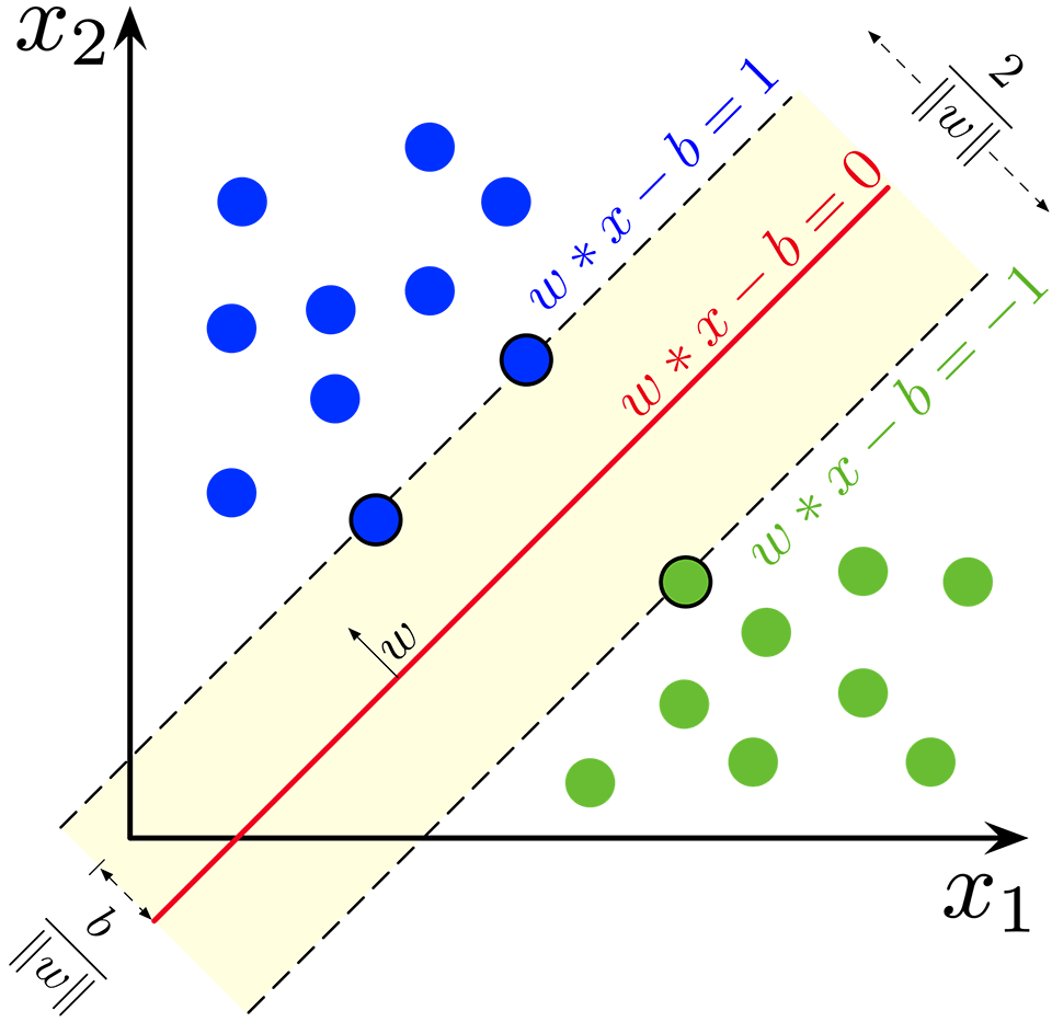
- Hyperplane: In a two-dimensional space, a hyperplane is a straight line. In higher dimensions, it becomes a plane.
- Margin: The space between the closest data points (support vectors) and the hyperplane.
The optimal hyperplane is the one that maximizes this margin. This concept is known as maximal margin classification.
SVMs are designed for datasets where the data points of different classes can be separated by a linear boundary.
For non-linearly separable datasets, SVMs become more versatile through approaches like kernel trick which introduces non-linearity to transform data into a higher-dimensional space before applying a linear classifier.
- Hinge Loss: SVMs utilize a hinge loss function that introduces a penalty when data points fall within a certain margin of the decision boundary. The goal is to correctly classify most data points while keeping the margin wide.
- Regularization: Another important aspect of SVMs is regularization, which balances between minimizing errors and maximizing the margin. This leads to a unique and well-defined solution.
An SVM minimizes the following loss function, subject to constraints:
Here,
A hyperplane in an
In a 2D space, the equation of a hyperplane is:
where
In the case of a linearly separable dataset, the
In a 2D space, the equation of a hyperplane is:
For example, for a hyperplane given by $w = \begin{bmatrix} 1 \ 2 \end{bmatrix}$ and
Here, the hyperplane is a line.
In a 3D space, the equation of a hyperplane is:
For example, for a hyperplane given by 

Here, the hyperplane is a plane.
The equation of a hyperplane in an
Here, the hyperplane is an
While the primal representation of SVM uses the direct equation of the hyperplane, the dual representation typically employs a kernel function to map the input to a higher-dimensional space. This approach avoids the need to explicitly compute the normal vector
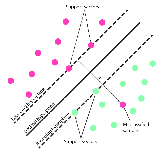
The Maximum Margin Classifier is the backbone of Support Vector Machines (SVM). This classifier selects a decision boundary that maximizes the margin between the classes it separates. Unlike traditional classifiers, which seek a boundary that best fits the data, the SVM finds a boundary with the largest possible buffer zone between classes.
Representing the decision boundary as a line, the classifier seeks to construct the "widest road" possible between points of the two classes. These points, known as support vectors, define the margin.
The goal is to find an optimal hyperplane that separates the data while maintaining the largest possible margin. Mathematically expressed:
Here,
The decision boundary, which is normalized to
The SVM also allows for a soft margin, introducing a regularization parameter
Here,
- Text Classification: SVMs with maximum margin classifiers are proficient in distinguishing spam from legitimate emails.
- Image Recognition: SVMs help in categorizing images by detecting edges, shapes, or patterns.
- Market Segmentation: SVMs assist in recognizing distinct customer groups based on various metrics for targeted marketing.
- Biomedical Studies: They play a role in the classification of biological molecules, for example, proteins.
To simplify, the model training aims to minimize the value:
This minimization task is executed using quadratic programming techniques, leading to an intricate but optimized hyperplane.
Support vectors play a central role in SVM, dictating the classifier's decision boundary. Let's see why they're crucial.
- Smart Learning: SVMs focus on data points close to the boundary that are the most challenging to classify. By concentrating on these points, the model becomes less susceptible to noise in the data.
- Computational Efficiency: Because the classifier is based only on the support vectors, predictions are faster. In some cases, most of the training data is not considered in the decision function. This is particularly useful in scenarios with large datasets.
During training, the SVM algorithm identifies support vectors from the entire dataset using a dual optimization strategy, called Lagrange multipliers. These vectors possess non-zero Lagrange multipliers, or dual coefficients, allowing them to dictate the decision boundary.
The decision boundary of an SVM is entirely determined by the support vectors that lie closest to it. All other data points are irrelevant to the boundary.
This relationship can be expressed as:
Where:
-
$i$ iterates over the support vectors -
$m$ represents the number of support vectors -
$\alpha_i$ and$y_i$ are the dual coefficients and the corresponding class labels, respectively -
$K(\mathbf{x}_i, \mathbf{x})$ is the kernel function -
$b$ is the bias term
Support Vector Machines (SVMs) are powerful supervised learning algorithms that can be used for both classification and regression tasks. One of their key strengths is their ability to handle both linear and non-linear relationships.
- Linear SVM: Maximizes the margin between the two classes, where the decision boundary is a hyperplane.
- Non-Linear SVM: Applies kernel trick which implicitly maps data to a higher dimensional space where a separating hyperplane might exist.
For linearly separable data, the decision boundary is defined as:
where
The margin (i.e., the distance between the classes and the decision boundary) is:
Optimizing linear SVMs involves maximizing this margin.
Non-linear SVMs apply the kernel trick, which allows them to indirectly compute the dot product of input vectors in a higher-dimensional space.
The decision boundary is given by:
where
Here is the Python code:
# Linear SVM
from sklearn.svm import SVC
linear_svm = SVC(kernel='linear')
linear_svm.fit(X_train, y_train)

# Non-Linear SVM with RBF kernel
rbf_svm = SVC(kernel='rbf')
rbf_svm.fit(X_train, y_train)To better understand how the Kernel Trick in SVM operates, let's start by reviewing a typical linear SVM representation.
The primal formulation:

where the first part of the above equation is the regularization term and the second part is the loss function.
We can write the Lagrangian for the constrained optimization problem as follows:

where
The dual expression has the form:
where
Now, let's consider the dual solution of the linear SVM problem in terms of the input data:
where $w^$ is the optimized weight vector, $\alpha_i^$ are the corresponding Lagrange multipliers, and
Using the Kernel Trick, we can rephrase
The kernelized representation of
where
Such a transformation allows the algorithm to operate in a higher-dimensional "kernel" space without explicitly mapping the data to that space, effectively utilizing the inner products in the transformed space.
By implementing the kernel trick, the decision function becomes:
where
The kernel trick thus enables SVM to fit nonlinear decision boundaries by employing various kernel functions, including:
-
Linear (no transformation):
$K(x, x') = x^T x'$ -
Polynomial:
$K(x, x') = (x^T x' + c)^d$ -
RBF:
$K(x, x') = \exp{\left(-\frac{|x - x'|^2}{2\sigma^2}\right)}$ -
Sigmoid:
$K(x, x') = \tanh(\kappa x^T x' + \Theta)$
Here is the Python code:
from sklearn.svm import SVC

# Initializing SVM with various kernel functions
svm_linear = SVC(kernel='linear')
svm_poly = SVC(kernel='poly', degree=3, coef0=1)
svm_rbf = SVC(kernel='rbf', gamma=0.7)
svm_sigmoid = SVC(kernel='sigmoid', coef0=1)

# Fitting the models
svm_linear.fit(X, y)
svm_poly.fit(X, y)
svm_rbf.fit(X, y)
svm_sigmoid.fit(X, y)The strength of Support Vector Machines (SVMs) comes from their ability to work in high-dimensional spaces while requiring only a subset of training data points, known as support vectors.
- Linear Kernel: Ideal for linearly separable datasets.
-
Polynomial Kernel: Suited for non-linear data and controlled by a parameter
$e$ . -
Radial Basis Function (RBF) Kernel: Effective for non-linear, separable data and influenced by a parameter
$\gamma$ . - Sigmoid Kernel: Often used in binary classification tasks, especially with neural networks.
While Linear Kernel is the simplest, RBF is the most versatile and widely used.
Here is the Python code:
from sklearn import datasets
from sklearn.model_selection import train_test_split
from sklearn.preprocessing import StandardScaler
from sklearn.svm import SVC
import numpy as np

# Load dataset
iris = datasets.load_iris()
X = iris.data
y = iris.target

# Make it binary
X = X[y != 0]
y = y[y != 0]

# Split dataset
X_train, X_test, y_train, y_test = train_test_split(X, y, test_size=0.2, random_state=42)

# Scale the features
scaler = StandardScaler()
X_train = scaler.fit_transform(X_train)
X_test = scaler.transform(X_test)

# Train and evaluate with different kernels
kernels = ['linear', 'poly', 'rbf', 'sigmoid']
for k in kernels:
    print(f"Evaluating with {k} kernel")
    clf = SVC(kernel=k, random_state=42)
    clf.fit(X_train, y_train)
    acc = clf.score(X_test, y_test)
print(f"Accuracy: {np.round(acc, 4)}")The soft margin technique in Support Vector Machines (SVM) allows for a margin that is not hard or strict. This can be beneficial when the data is not perfectly separable. The "C" parameter is instrumental in controlling the soft margin, also known as the regularization parameter.
In practical settings, datasets are often not perfectly linearly separable. In such cases, a hard margin (RBF kernel for example) can lead to overfitting and degraded generalization performance. The soft margin, in contrast, can handle noise and minor outliers more gracefully.
Rather than seeking the hyperplane that maximizes the margin without any misclassifications (as in a hard margin), a soft margin allows some data points to fall within a certain distance from the separating hyperplane.
The choice of which points can be within this "soft" margin is guided by the concept of slack variables, denoted by
In the context of the soft margin, slack variables are used to quantify the classification errors and their deviation from the decision boundary. Mathematically, the margin for each training point is
The goal is to find the optimal hyperplane while keeping the sum of slack variables (
This formulation represents a trade-off between maximizing the margin and minimizing the sum of the slack variables (
Here is the Python code:
from sklearn import datasets
from sklearn.svm import SVC
import numpy as np

# Generate a dataset that's not linearly separable
X, y = datasets.make_moons(noise=0.3, random_state=42)

# Fit a hard margin (linear kernel) SVM
# Notice the error; the hard margin cannot handle this dataset
svm_hard = SVC(kernel="linear", C=1e5)
svm_hard.fit(X, y)

# Compare with a soft margin (linear kernel) SVM
svm_soft = SVC(kernel="linear", C=0.1)  # Using a small C for a more soft margin
svm_soft.fit(X, y)

# Visualize the decision boundary for both
# (Visual interface can better demonstrate the effect of C)Support Vector Machines (SVMs) are inherently binary classifiers, but they can effectively perform multi-class classification using a suite of strategies.
-
One-Vs.-Rest (OvR):
- Each class has its own classifier which is trained to distinguish that class from all others. During prediction, the class with the highest confidence from their respective classifiers is chosen.
-
One-Vs.-One (OvO):
- For
$k$ classes,$\frac{{k \times (k-1)}}{2}$ classifiers are trained, each distinguishing between two classes. The class that "wins" the most binary classifications is the predicted class.
- For
-
Decision-Tree-SVM Hybrid:
- Builds a decision tree on top of SVMs to handle multi-class problems. Each leaf in the tree represents a class and the path from the root to the leaf gives the decision.
-
Error-Correcting Output Codes (ECOC):
- Decomposes the multi-class problem into a series of binary ones. The codewords for the binary classifiers are generated such that they correct errors more effectively.
-
Direct Multi-Class Approaches: Modern SVM libraries often have built-in algorithms that allow them to directly handle multi-class problems without needing to decompose them into multiple binary classification problems.
Here is the Python code:
from sklearn.svm import SVC
from sklearn.multiclass import OneVsRestClassifier, OneVsOneClassifier
from sklearn.tree import DecisionTreeClassifier
from sklearn.datasets import load_iris
from sklearn.model_selection import train_test_split
from sklearn.metrics import accuracy_score, classification_report

# Load the Iris dataset
iris = load_iris()
X, y = iris.data, iris.target

# Split the data into training and testing sets
X_train, X_test, y_train, y_test = train_test_split(X, y, test_size=0.3, random_state=42)

# Initialize different multi-class SVM classifiers
svm_ovo = SVC(decision_function_shape='ovo')
svm_ovr = SVC(decision_function_shape='ovr')
svm_tree = DecisionTreeClassifier()
svm_ecoc = SVC(decision_function_shape='ovr')

# Initialize the OvR and OvO classifiers
ovr_classifier = OneVsRestClassifier(SVC())
ovo_classifier = OneVsOneClassifier(SVC())

# Train the classifiers
svm_ovo.fit(X_train, y_train)
svm_ovr.fit(X_train, y_train)
svm_tree.fit(X_train, y_train)
svm_ecoc.fit(X_train, y_train)
ovr_classifier.fit(X_train, y_train)
ovo_classifier.fit(X_train, y_train)

# Evaluate each classifier
classifiers = [svm_ovo, svm_ovr, svm_tree, svm_ecoc, ovr_classifier, ovo_classifier]
for clf in classifiers:
    y_pred = clf.predict(X_test)
    accuracy = accuracy_score(y_test, y_pred)
    print(f"Accuracy using {clf.__class__.__name__}: {accuracy:.2f}")

# Using the prediction approach for different classifiers
print("\nClassification Report using different strategies:")
for clf in classifiers:
    y_pred = clf.predict(X_test)
    report = classification_report(y_test, y_pred, target_names=iris.target_names)
print(f"{clf.__class__.__name__}:\n{report}")While Support Vector Machines (SVMs) are powerful tools, they do come with some limitations.
The primary algorithm for finding the optimal hyperplane, the Sequential Minimal Optimization algorithm, has a worst-case time complexity of
SVMs can be sensitive to the choice of hyperparameters, such as the regularization parameter (C) and the choice of kernel. It can be a non-trivial task to identify the most appropriate values, and different datasets might require different settings to achieve the best performance, potentially leading to overfitting or underfitting.
The SVM fitting procedure generally involves storing the entire dataset in memory. Moreover, the prediction process can be CPU-intensive due to the need to calculate the distance of all data points from the decision boundary.
SVMs, in their basic form, are designed to handle linearly separable data. While kernel methods can be employed to handle non-linear data, interpreting the results in such cases can be challenging.
While some SVM implementations provide tools to estimate probabilities, this is not the algorithm's native capability.
Given their resource-intensive nature, SVMs are not well-suited for very large datasets. Additionally, the absence of a built-in method for feature selection means that feature engineering needs to be comprehensive before feeding the data to an SVM model.
SVMs are fundamentally binary classifiers. While there are strategies such as One-Vs-Rest and One-Vs-One to extend their use to multi-class problems, these approaches come with their own sets of caveats.
Selecting the optimal kernel function can be challenging, especially without a good understanding of the data's underlying structure.
SVMs can be adversely affected by noisy data or datasets where classes are not distinctly separable. This behavior can lead to poor generalization on unseen data.
The Support Vector Machine (SVM) employs a hinge loss that serves as its objective function.
The hinge loss is a piecewise function, considering the margin's distance to the correct classification for
And particularly in the SVM context:
Where:
-
$z$ represents the product$y_i \cdot f(x_i)$ . -
$y_i$ is the actual class label, either -1 or 1. -
$f(x_i)$ is the decision function or score computed by the SVM model for data point$x_i$ .
The hinge loss is graphically characterized by a zero loss for values
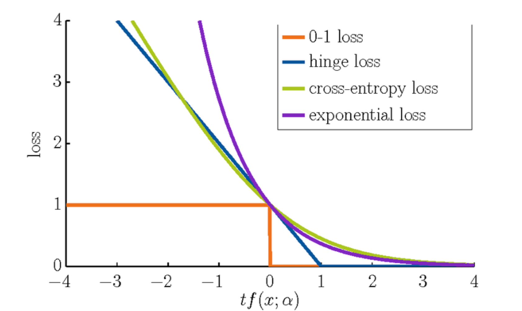
From a mathematical standpoint, the hinge loss function
The Empirical Risk Minimization (ERM) of the SVM involves the following optimization problem of minimizing the sum of hinge losses over all data points:
Subject to:
Where:
-
$C$ is a regularization parameter, balancing margin maximization with training errors. -
$w$ is the weight vector. -
$b$ is the bias term.
Here is the Python code:
import numpy as np

def hinge_loss(y, f_x):
    return np.maximum(0, 1 - y * f_x)

# Example calculation
y_true = 1
f_x = 0.5
loss = hinge_loss(y_true, f_x)
print(f"Hinge loss for f(x) = {f_x} and true label y = {y_true}: {loss}")The Lagrange multipliers, central to the concept of Support Vector Machines (SVM), are introduced to handle the specifics of constrained optimization.
-
Optimization Objective: SVM aims to maximize the margin, which involves balancing the margin width and the training error. This is formalized as a quadratic optimization problem.
-
Decision Boundary: The optimized hyperplane produced by SVM acts as the decision boundary.
-
Support Vectors: These are the training data points that lie closest to the decision boundary. The classifier's performance is dependent only on these points, leading to the sparse solution behavior.
The use of Lagrange multipliers is a defining characteristic of SVMs, offering a systematic way to transform a constrained optimization problem into an unconstrained one. This transformation is essential to construct the linear decision boundary and simultaneously determine the set of points that contribute to it.
Let's define the key terms:
-
$\mathbf{w}$ and$b$ are the parameters of the hyperplane. -
$\xi_i$ are non-negative slack variables.
The primal problem can be formulated as:

The associated Lagrangian function is:

Terms involving
By setting the derivatives of
Solving the Dual Problem when optimizing a Support Vector Machine (SVM) allows for more efficient computation and computational tractability through the use of optimization techniques like the Lagrange multipliers and Wolfe dual.
-
Lagrange Duality: The process aims to convert the primal (original) optimization problem into a dual problem, which is simpler and often more computationally efficient. This is achieved by introducing Lagrange multipliers, which are used to form the Lagrangian.
-
Karush-Kuhn-Tucker (KKT) Conditions: The solution to the dual problem also satisfies the KKT conditions, which are necessary for an optimal solution to both the primal and dual problems.
-
Wolfe Duality: Works in conjunction with KKT conditions to ensure that the dual solution provides a valid lower bound to the primal solution.
-
Formulate the Lagrangian: Combine the original optimization problem with the inequality constraints using Lagrange multipliers.
-
Compute Partial Derivatives: Calculate the partial derivatives of the Lagrangian with respect to the primal variables, and set them equal to zero.
-
Determine KKT Violations: At the optimum, the differentiability conditions should be met. Check for KKT violations, such as non-negativity of the Lagrange multipliers and complementary slackness.
-
Simplify the Dual Problem:
- Substitute the primal variables using the KKT optimality conditions.
- Arrive at the expression for the Wolfe dual, which provides a lower bound to the primal objective function.
-
Solve the Dual Problem: Often using mathematical techniques or computational tools to find the optimal dual variables, or Lagrange multipliers, which correspond to optimal separation between classes.
-
Recover the Primal Variables: Using the KKT conditions, one can reconstruct the solution to the primal problem, typically involving the support vectors.
Here is the Python code:
import numpy as np
from sklearn import datasets
from sklearn.preprocessing import StandardScaler
from sklearn.svm import SVC

# Load Iris dataset
iris = datasets.load_iris()
X = iris.data
y = iris.target

# Feature scaling and data preparation
scaler = StandardScaler().fit(X)
X = scaler.transform(X)

# Fit linear SVM
svm = SVC(kernel='linear', C=1.0).fit(X, y)

# Computing support vectors and dual coefficients
support_vectors = svm.support_vectors_
dual_coefficients = np.abs(svm.dual_coef_)

# Recovering the primal coefficients and intercept
primal_coefficients = np.dot(dual_coefficients, support_vectors)
intercept = svm.intercept_

# Printing results
print("Support Vectors:\n", support_vectors)
print("Dual Coefficients:\n", dual_coefficients)
print("Primal Coefficients:", primal_coefficients)
print("Intercept:", intercept)Choosing the regularization parameter
-
Model Parameters: Learned from data during training, such as weights in linear regression.
-
Hyperparameters: Set before the learning process and are not learned from data.
Optimizing model hyperparameters like
-
$C$ : Trades off correct classification of training points against the maximal margin. A smaller$C$ encourages a larger margin. -
$\gamma$ in RBF Kernel: Sets the 'spread' of the kernel. Higher values lead to tighter fits of the training data. -
Choice of Kernel: Modifies the optimization problem.
-
Kernel Parameters: Each kernel may have specific hyperparameters.
-
Grid Search: Checks all possible hyperparameter combinations, making it exhaustive but computationally expensive.
-
Random Search: Randomly samples from a hyperparameter space, which can be more efficient and effective in high dimensions.
-
Bayesian Optimization: Utilizes results of past evaluations to adaptively pick the next set of hyperparameters. This often results in quicker convergence.
-
Genetic Algorithms: Simulates natural selection to find the best hyperparameters over iterations.
-
Train-Validation-Test Split: Used to manage overfitting when tuning hyperparameters.
-
Cross-Validation: A more robust method for tuning hyperparameters.
- Accuracy: The percentage of correct predictions.
- Precision: The ability of the classifier not to label as positive a sample that is negative.
- Recall: The ability of the classifier to find all the positive samples.
- F1 Score: The weighted average of Precision and Recall.
Here is the code:
from sklearn.model_selection import GridSearchCV
from sklearn import svm, datasets

# Load dataset
iris = datasets.load_iris()
X, y = iris.data, iris.target

# Specify the hyperparameter space
param_grid = {'C': [0.1, 1, 10, 100]}

# Instantiate the model
svc = svm.SVC()

# Set up the grid search
grid_search = GridSearchCV(svc, param_grid, cv=5)

# Perform the grid search
grid_search.fit(X, y)

# Get the best parameter
best_C = grid_search.best_params_['C']
print(f"The best value of C is {best_C}")The hinge loss function is a key element in optimizing Support Vector Machines (SVMs). It's a non-linear loss function that's singularly focused on classification rather than probability. In mathematical terms, the hinge loss function is defined as:
Here,
The hinge loss function corresponds to the margin distance between the decision boundary and the support vectors:
- When a point is correctly classified and beyond the margin, the hinge loss is zero.
- When a point is within the margin, the classifier is penalized proportionally to how close the point is to the margin, ensuring the decision boundary separates the classes.
- If a point is misclassified, the hinge loss is positive and directly proportional to the distance from the decision boundary.
This geometric interpretation aligns with the goal of SVMs: to find the hyperplane that maximizes the margin while minimizing the hinge loss.
Explore all 70 answers here 👉 Devinterview.io - SVM