44 Essential Q-Learning Interview Questions

You can also find all 44 answers here 👉 Devinterview.io - Q-Learning

1. What is Q-learning, and how does it fit in the field of reinforcement learning?

Q-Learning is a central algorithm in Reinforcement Learning, renowned for its ability to learn optimal strategies. One of its strengths lies in its versatility across different domains, from games to real-world scenarios.

Reinforcement Learning: Building Blocks

Reinforcement Learning revolves around an agent that takes actions within an environment to maximize a cumulative reward. Both the agent and the environment interact in discrete time steps.

At each time step $t$:

• The agent selects an action $a_t$ based on a chosen strategy.
• The environment transitions to a new state $s_{t+1}$, and the agent receives a numerical reward $r_{t+1}$ as feedback.

The core challenge is to develop a strategy that ensures the agent selects actions to maximize its long-term rewards.

Q-Learning: Adaptive Strategy

With Q-learning, the agent learns how good it is to take a specific action in a particular state (by computing the action's Q-value), then chooses the action with the highest Q-value.

1. Q-Value Iteration:

   • Initialization: Start with arbitrary Q-values.
   • Value Iteration: Update Q-values iteratively, aligning them with empirical experiences.
   • Convergence: The process continues until Q-values stabilize.

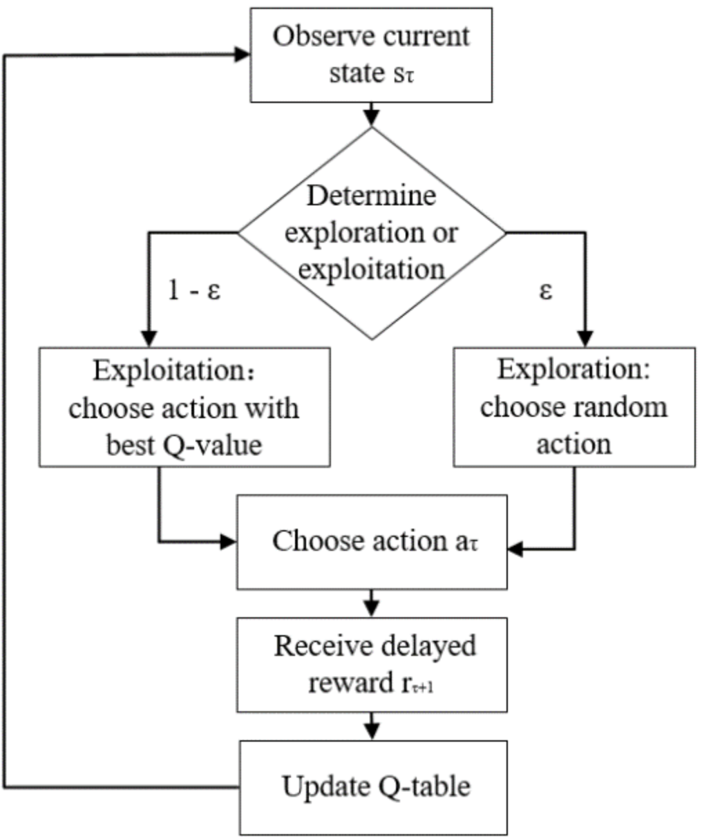
2. Action Selection Based on Q-Values: Use an exploration-exploitation strategy, typically ε-greedy, where the agent chooses the best action (based on Q-values) with probability $1 - \epsilon$, and explores with probability $\epsilon$.

Core Mechanism

The updated Q-value for a state-action pair $Q(s_t, a_t)$ is calculated using the classic Bellman Equation:

$$ Q(s_t, a_t) \leftarrow (1 - \alpha) \cdot Q(s_t, a_t) + \alpha \cdot \left( r_t + \gamma \cdot \max_a Q(s_{t+1}, a) \right) $$

Here: $\alpha$ represents the learning rate, determining the extent to which new information replaces old. $\gamma$ is the discount factor that balances immediate and long-term rewards.

Exploration vs. Exploitation

• Exploration is vital to encounter new state-action pairs that may lead to better long-term rewards.
• Exploitation utilizes existing knowledge to select immediate best actions.

A well-calibrated ε-greedy strategy resolves this trade-off.

Practical Applications

• Games: Q-learning has excelled in games like Tic-Tac-Toe, Backgammon, and more recently, in beating champions in complex domains such as Go and Dota 2.
• Robotics: It's been used to train robots for object manipulation and navigation.
• Finance: Q-learning finds application in portfolio management and market prediction.
• Telecommunication: For optimizing routing and data transfer in networks.
• Healthcare: To model patient treatment plans.

Optimality and Convergence

Under certain conditions, Q-learning is guaranteed to converge to the optimal Q-values and policy:

1. Finite Exploration: All state-action pairs are visited an infinite number of times.
2. Decaying Learning Rate: The learning rate $\alpha$ diminishes over time, allowing older experiences to hold more weight.

Code Example: Q-Learning for Gridworld

Here is a Python code.

import numpy as np
import random

# Initialize Q-table
q_table = np.zeros([grid_size, grid_size, num_actions])

# Q-learning parameters
alpha = 0.1
gamma = 0.9
epsilon = 0.1

# Exploration-exploitation for action selection
def select_action(state, epsilon):
    if random.uniform(0, 1) < epsilon:
        return random.choice(possible_actions)
    else:
        return np.argmax(q_table[state])

# Q-value update
def update_q_table(state, action, reward, next_state):
    q_value = q_table[state][action]
    max_next_q_value = np.max(q_table[next_state])
    new_q_value = (1 - alpha) * q_value + alpha * (reward + gamma * max_next_q_value)
    q_table[state][action] = new_q_value

2. Can you describe the concept of the Q-table in Q-learning?

The Q-table lies at the core of the Q-learning algorithm, serving as the primary mechanism through which the agent learns and refines its action-selection policy for different states.

Purpose

The Q-table records the Q-values for every state-action pair, representing the cumulative expected reward the agent associates with taking an action in a specific state. This data forms the basis for the agent to make optimal decisions, balancing immediate rewards and potential long-term gain.

Storage Requirements

Inconsistent with the curse of dimensionality, the Q-table's storage increases with more complex state and action spaces—often rendering it impractical for large-scale, real-world tasks.

Q-Learning Algorithm Updates

The Q-table is dynamically updated using the Bellman equation during the agent's exploration and experience gathering.

• Direct Update: After executing an action and observing the resultant reward and new state, the Q-value is updated using the formula:

$$ Q(s_t, a_t) \leftarrow Q(s_t, a_t) + \alpha \cdot \left( r_t + \gamma \cdot \max_a Q(s_{t+1}, a) - Q(s_t, a_t) \right) $$

Here, $\alpha$ represents the learning rate (balancing new information and past knowledge), and $\gamma$ is the discount factor (present-future reward trade-off).

• Exploration-Guided Update: If the agent follows a random exploration action and receives a reward, the Q-value updates are slightly adjusted:

$$ Q(s_t, a_t) \leftarrow Q(s_t, a_t) + \alpha \cdot \left( r_t - Q(s_t, a_t) \right) $$

Policy Decisions

Each round, the epsilon-greedy strategy leverages the Q-values stored in the table, combined with a degree of exploration, to guide the agent in selecting an action.

• With probability $\epsilon$, the agent explores randomly, aiming to update or enhance its Q-table.
• Otherwise, with probability $1 - \epsilon$, the agent exploits past knowledge by selecting the action with the highest Q-value.

Code Example: Updating the Q-Table

Here is the Python code:

# Assuming alpha, gamma, and epsilon are defined

# Direct Update
Q[state][action] += alpha * (reward + gamma * max(Q[new_state]) - Q[state][action])

# Exploration-Guided Update
if random.uniform(0, 1) < epsilon:
    Q[state][action] += alpha * (reward - Q[state][action])

3. How does Q-learning differ from other types of reinforcement learning such as policy gradient methods?

Q-Learning leverages the concept of an action-value function $Q$ to make decisions and learn from them. It uses an exploration-exploitation strategy to balance the trade-off between choosing known good actions and exploring new ones.

In contrast, techniques such as policy gradient methods directly approximate the policy function $\pi(a|s)$, which maps states to actions, usually in a stochastic manner. This approach continuously improves the policy based on observed rewards and often employs temporal difference learning.

Key Differences

Q Function vs. Policy Function

• Q-Learning: Focuses on the $Q$ function, which estimates the expected cumulative reward of taking action $a$ in state $s$ and following a particular strategy thereafter. The agent selects actions that maximize $Q$ for the current state.
• Policy Gradient Methods: Directly approximates the policy function $\pi(a|s)$, which represents the probability of taking action $a$ in state $s$. The agent samples actions from this distribution.

Exploration Methods

• Q-Learning: Incorporates a balance between exploration and exploitation through strategies like $\epsilon$-greedy, where the agent chooses the best known action most of the time but also explores with a small probability $\epsilon$.
• Policy Gradient Methods: Often uses a softmax strategy to encourage exploration, where actions are selected based on their probabilities as determined by the policy function.

Convergence Speed

• Q-Learning: The $Q$ function is directly optimized to approximate the optimal action-value function. This can lead to quicker convergence, especially in deterministic environments.
• Policy Gradient Methods: The policy function might require more iterations to converge to the optimal policy. However, in stochastic or high-dimensional action spaces, policy gradient methods can be more effective.

Computational Complexity

• Q-Learning: The primary computational task is updating the $Q$ values, which becomes simpler with tabular methods. In discrete and small state and action spaces, $Q$-learning can be highly efficient.
• Policy Gradient Methods: These methods calculate gradients, which could be computationally expensive, especially in scenarios with continuous actions.

Model Requirement

• Q-Learning: Does not require knowledge of or reliance on an underlying environment model, making it more suitable for model-free settings.
• Policy Gradient Methods: Can operate in both model-free and model-based environments, and their performance can benefit from such models.

4. Explain what is meant by the term 'action-value function' in the context of Q-learning.

The action-value function $Q(s, a)$ is a core concept in Q-learning. It carries the most up-to-date information about which actions lead to the highest cumulative rewards in a given state.

Mathematical Representation

The action-value function is a map from a state-action pair $(s, a)$ to a value that communicates the utility or long-term potential of an action within a specific state:

$$ Q(s, a) = \mathbb{E} \left[ R_t | s, a \right] $$

Where:

• $R_t$ is the expected cumulative reward or $G_t$, related to action $a$ and the following trajectory.
• The expectation represents the mean of the rewards under certain conditions.

Practical Usage

• Policy Selection: The action $a'$ that achieves the highest $Q(s, a')$ is typically selected.
• Model-Free Approach: Suitable in environments where transition probabilities $P(s' | s, a)$ or expected rewards $\mathbb{E}(R | s, a)$ are unknown.
• Updated via Temporal Difference: Utilizing the Bellman Equation, the action-value function is refined through observed rewards and potential future rewards, adapting it iteratively toward a more accurate approximation.

Algorithm: Q-Learning

This classic temporal difference learning method estimates the action-value function through direct experience (environment interaction).

1. Initialization

   • Begin with a table or approximate function for $Q(s, a)$ (e.g., a neural network in deep Q-learning).

2. Action Selection

   • Using exploration-exploitation strategies, such as $\epsilon$-greedy, select an action to execute in the current state $s$.

3. Learning from Experience

   • Observe the reward $R$ and the resulting state $s'$.
   • Update the $Q(s, a)$ estimate based on:
     • The observed reward.
     • The best $Q$ estimate for the next action in the following state.
     • A learning rate and a discount factor to control update dynamics and reward importance.

4. Convergence and Policy Derivation

   • Over many interactions, the $Q(s, a)$ values approximate the true action-value function. The action that maximizes the learned $Q$ at each state becomes the policy.

5. Loop

   • Continue exploring the environment, updating $Q$, and refining the policy.

Code Example: Action-Value Update

Here is the Python code:

# Initialize a dictionary to represent the action-value function
Q = {}
state = 's1'
action = 'a1'
reward = 1
next_state = 's2'
alpha = 0.1  # learning rate
gamma = 0.9  # discount factor

# Update the action-value function for the state-action pair (s1, a1)
Q[state, action] = Q.get((state, action), 0) + alpha * (reward + gamma * max([Q.get((next_state, a), 0) for a in possible_actions]) - Q.get((state, action), 0))

print(Q)

5. Describe the role of the learning rate (α) and discount factor (γ) in the Q-learning algorithm.

In Q-Learning, the learning rate $\alpha$ and the discount factor $\gamma$ play vital roles in updating the Q-values.

Learning Rate: $\alpha$

The learning rate $\alpha$ determines the speed and magnitude at which the Q-values are updated during the learning process.

• Update Formula:

$$ Q(s_t, a_t) \leftarrow (1 - \alpha) \cdot Q(s_t, a_t) + \alpha \cdot (r_{t+1} + \gamma \cdot \max_a Q(s_{t+1}, a)) $$

• Effect on Exploration vs. Exploitation:
  • When $\alpha$ is high, Q-values are updated significantly, leading to more exploration.
  • Lower $\alpha$ values lean towards exploitation by being less open to changing the Q-values.

Discount Factor: $\gamma$

The discount factor $\gamma$ shapes the agent's behavior by balancing immediate and future rewards.

• Update Formula:

$$ Q(s, a) \leftarrow (1 - \alpha) \cdot Q(s, a) + \alpha \cdot (r + \gamma \cdot \max_{a'} Q(s', a')) $$

• Role in Delayed Rewards: A value of $\gamma < 1$ ensures the agent considers future rewards but with a diminishing focus. A lower $\gamma$ puts more emphasis on immediate rewards.

Code Example: Learning Rate and Discount Factor

Here is the Python code:

# Parameters
alpha = 0.5        # Learning rate
gamma = 0.9        # Discount factor

# Q-Value Update
Q[state][action] = (1 - alpha) * Q[state][action] + alpha * (reward + gamma * max_future_q)

6. What is the exploration-exploitation trade-off in Q-learning, and how is it typically handled?

Balancing exploration and exploitation is central to the success of Q-Learning and other reinforcement learning algorithms.

Exploration vs. Exploitation

• Exploration: Involves acting randomly or trying out different strategies to gain information about the environment, potentially sacrificing short-term rewards.

• Exploitation: It leverages already-acquired knowledge to select actions that are likely to yield high short-term rewards, based on the best action known so far for each state.

$Q$-Value Mechanics

The $Q$-function quantifies the quality of an action in a specific state. During learning, it gets updated to better estimate the long-term reward of taking that action from that state.

The update is a combination of the current $Q$-value, the instant reward, and a discounted estimate of the best achievable future reward:

$$ Q(s_t, a_t) \leftarrow (1 - \alpha) \cdot Q(s_t, a_t) + \alpha \cdot \left( R_{t+1} + \gamma \cdot \max_a Q(s_{t+1}, a) \right) $$

• $\alpha$: The learning rate, determining to what extent new information overrides old.

• $\gamma$: The discount factor, emphasizing immediate rewards over delayed ones ($0$ for purely myopic strategies, $1$ for long-term focus).

Handling Exploration-Exploitation

Several strategies balance these two competing objectives.

1. Epsilon-Greedy: The agent picks a random action with probability $\varepsilon$ (exploration) and the action with the highest $Q$-value with probability $1 - \varepsilon$ (exploitation).

2. Softmax Action Selection: Also known as the Boltzmann exploration-exploitation algorithm, this methods selects actions probabilistically, with the probabilities proportional to the exponentials of the Q-values.

3. Upper-Confidence Bound (UCB): It's based on the principle of optimism in the face of uncertainty. The agent picks an action based on both its current estimate of the action's value and the uncertainty in that estimate.

4. Thompson Sampling: A Bayesian approach where the agent maintains a probability distribution over each action's $Q$-value. The agent samples from those distributions and acts greedily with respect to the sampled values.

5. Dynamic $Q$-Learning Strategies: These strategies alter the exploration rate ($\varepsilon$) over time, typically starting with a higher exploration rate and reducing it as the system learns more. Some methods include linear, logarithmic, or exponential decay.

Code Example: Epsilon-Greedy

Here is the Python code:

import random

epsilon = 0.1  # Example epsilon value for 10% exploration

def epsilon_greedy(state, q_table):
    if random.uniform(0, 1) < epsilon:  # Exploration
        return random.choice(possible_actions)
    else:  # Exploitation
        return max(q_table[state], key=q_table[state].get)

7. Define what an episode is in the context of Q-learning.

In the context of Q-Learning, an episode refers to the full sequence that the agent takes, starting from an initial state, making decisions based on the current Q-values, interacting with the environment and receiving corresponding rewards, until reaching a terminal state.

Key Concepts

• SARSA: The agent learns and makes decisions using the state-action-reward transition during this episode.

• Q-Learning: The agent records state-action rewards and updates the Q-table after the episode, even if the episode isn't complete. This technique is known as off-policy learning.

Code Example: Single Episode

Here is the Python code:

import numpy as np

# Initialize Q-table
q_table = np.zeros([num_states, num_actions])

# Set hyperparameters
alpha = 0.1
gamma = 0.6
epsilon = 0.1

# Choose initial state
state = 1

# Episode loop
while not done:
    # Select an action using epsilon-greedy
    action = epsilon_greedy(q_table, state, epsilon)
    
    # Take the action and observe the new state and reward
    next_state, reward, done, info = env.step(action)
    
    # Update Q-value using the Q-learning equation
    current_q = q_table[state, action]
    max_next_q = np.max(q_table[next_state])
    new_q = (1 - alpha) * current_q + alpha * (reward + gamma * max_next_q)
    q_table[state, action] = new_q
    
    # Update the state
    state = next_state

8. Discuss the concept of state and action space in Q-learning.

In Q-Learning, an agent learns to make decisions by interacting with an environment. The learning process is essentially a balance between exploration to gather new experiences and exploitation to maximize rewards.

Central to this learning is the concept of state $s$ which represents a unique configuration or observation of the environment, and action $a$ which is a decision the agent can make from a given state.

Tackling Complexity with State and Action Spaces

In real-world scenarios, environments can be complex and dynamic. For instance, in robotic navigation, a robot might have numerous potential positions and directions to move in. Both the navigation needs and the physical mechanism constrains the robot. In a video game setting, the agent might have to navigate a maze to reach a goal.

This is where the notions of state and action spaces in Q-Learning come into play. They're mechanisms for constraining the learning process, both practically and computationally, and facilitating the delineation of optimal strategies by the agent.

Action Space

The action space, denoted as $A$, is the set of all possible actions that the agent can take in any given state. While this can often be a straightforward set of actions such as "move left, right, up, down" or more complex like "select a point on a continuous spectrum," the Q-Learning algorithm uses a lookup table structure (Q-table) to keep track of the learned utility values for each state-action pair.

The action space is crucial in the context of the exploitation strategy. Upon entering a state, the agent refers to the Q-table to choose the action with the highest associated utility.

Code Example: Discrete Action Space

Here is the Python code:

# Defining the action space
action_space = ['up', 'down', 'left', 'right', 'jump']

# Q-table will store Q-values for each state-action pair
Q_table = {(state, action): 0 for state in state_space for action in action_space}

State Space

The state space, denoted as $S$, is the collection of all possible states the environment can occupy. How these states are defined greatly influence the learning process.

In many applications, the state space can be discrete, comprising a finite or countably infinite number of distinct, well-defined states. For instance, in a game of tic-tac-toe, the state space is clearly delineated by whether each cell in the 3x3 grid is occupied by a player's marker, and if so, whose marker it is.

On the other hand, a state space can be continuous, which is the case when a state cannot be uniquely or directly associated with a discrete value or category. For example, in a robotics control task, the state might be described by the real-valued joint angles of the robot, and its urban environment could be represented in continuous space.

Ensuring the agent can explore and learn effectively in both discrete and continuous state spaces can be a challenge. This is where Q-Learning algorithms, including their more sophisticated derivatives like Deep Q-Networks, come into play to tackle challenging learning tasks.

The Q-learning iterations help form a Q-function, denoted as Q(s, a). It represents the expected cumulative reward the agent can achieve by taking action $a$ when in state $s$. When the agent interacts with the environment, it will update these Q-values to provide better decision-making in future interactions.

For recurrent or continuing tasks, Q-learning algorithms can balance exploration and exploitation through exploration strategies which can minimize the exploration-exploitation tradeoff where usually increasing either will decrease the other.

9. Describe the process of updating the Q-values in Q-learning.

Q-Learning typically uses the following approach to update $Q$-values:

Generalized Update Equation

$$ Q(s_t, a_t) \leftarrow Q(s_t, a_t) + \alpha \left(r_t + \gamma \max\limits_{a} Q(s_{t+1}, a) - Q(s_t, a_t)\right) $$

Here, $\alpha$ is the learning rate, $\gamma$ is the discount factor, $s_t$ and $a_t$ are the current state and the action chosen in that state, and $s_{t+1}$ is the next state.

Step-by-Step Update

1. Obtain Immediate Reward

   After agent $k$ takes action $a_k$ in state $s_k$, the environment provides the immediate reward $r_k$.

2. Update the Q-Value

$$ Q(s_k, a_k) \leftarrow (1 - \alpha) \times Q(s_k, a_k) + \alpha \times \left( r_k + \gamma \times \max\limits_{a} Q(s_{k+1}, a) \right) $$

Here, $\alpha$ is the learning rate, $s_k$ is the current state, and $a_k$ is the action chosen in that state.

3. Rinse and Repeat

   The process continues iteratively as the agent explores the environment.

10. What is the Bellman Equation, and how does it relate to Q-learning?

At the heart of Q-Learning is the Bellman Equation, a fundamental concept that drives the iterative process of updating Q-values based on experience.

The Bellman Equation

The Bellman Equation for the action-value function (Q-function) is as follows:

$$ Q^{\pi}(s,a) = E\left[ r + \gamma \max_{a'} Q^{\pi}(s', a') , \middle| , s, a \right] $$

Here's what each term means:

• $Q^{\pi}(s,a)$: The expected return, starting from state $s$, taking action $a$, and then following policy $\pi$.

• $r$: The immediate reward after taking action $a$ in state $s$.

• $\gamma$: The discount factor, which balances immediate and future rewards.

• $\max_{a'} Q^{\pi}(s', a')$: The maximum expected return achievable from the next state $s'$, considering all possible actions.

• $E$: The expectation operator, representing the long-term return, which embodies the Markov Decision Process (MDP).

The Bellman Equation states that the expected return from a state-action pair is the sum of the immediate reward and the discounted maximum expected return from the next state.

Deriving the Q-Learning Update Rule

By re-arranging the Bellman Equation, we get the Q-value iterative update rule, which is foundational to Q-Learning:

$$ Q(s, a) \leftarrow Q(s, a) + \alpha \left( r + \gamma \max_{a'} Q(s', a') - Q(s, a) \right) $$

Here, $\alpha$ represents the learning rate, which determines the extent to which new information overrides existing Q-values.

Key Q-Learning Components

1. Exploration-Exploitation Dilemma: Balancing between trying new actions (exploration) and selecting actions based on current knowledge (exploitation). This is typically achieved using $\epsilon$-greedy strategies.

2. Temporal Difference (TD) Error: It represents the discrepancy between the actual reward and the expected reward, serving as the basis for updating the Q-value. It's given by:

$$ \text{TD-error} = r + \gamma \max_{a'} Q(s', a') - Q(s, a) $$

Code Example: Q-Learning Update

Here is the Python code:

# Initialize Q-table
Q = np.zeros([num_states, num_actions])

# Define update hyperparameters
learning_rate = 0.1
discount_factor = 0.9

# Choose an action using ε-greedy
action = epsilon_greedy(Q, state, epsilon)

# Take the action, observe the reward and next state
next_state, reward = environment.step(action)

# Compute TD-error
td_error = reward + discount_factor * np.max(Q[next_state]) - Q[state, action]

# Update Q-value
Q[state, action] += learning_rate * td_error

11. Explain the importance of convergence in Q-learning. How is it achieved?

Q-Learning uses an iterative approach to converge towards the optimal action-value function $Q^*(s, a)$. Convergence ensures that the policy derived from the action-value function is optimal.

Importance of Convergence

• Stability: Without convergence, Q-values can keep oscillating, leading to unreliable and sub-optimal policies.

• Efficiency: Convergence helps Q-learning achieve optimality in a finite, albeit potentially large, number of iterations.

Achieving Convergence

• Exploration vs. Exploitation: A balanced approach is needed for the agent to visit and learn from all state-action pairs. This is often achieved using strategies like epsilon-greedy.

• Learning Rate ($\alpha$): By annealing or keeping learning rates small, Q-values are updated gradually, allowing the agent to explore more while fine-tuning.

• Discount Factor ($\gamma$): Encourages the agent to look further into the future. However, having a discount factor that's too high can lead to slow convergence.

• Initial Q-Values: Setting initial Q-values to 0 or another small value can help promote exploration early in learning.

• Environment Properties: Some environments may naturally lend themselves to quicker or slower convergence. For instance, in a highly stochastic environment vs. a deterministic one, the former might take longer to converge.

Python Example: Q-Learning Convergence

Here is the Python code:

import numpy as np

# Initialize Q-Table
Q = np.zeros([num_states, num_actions])

# Q-Learning Parameters
alpha = 0.1  # Learning Rate
gamma = 0.9  # Discount Factor
epsilon = 0.1  # Probability of Exploration

# Q-Learning Algorithm
for episode in range(num_episodes):
    state = env.reset()
    done = False
    while not done:
        # Choose Action
        if np.random.uniform(0, 1) < epsilon:
            action = env.action_space.sample()  # Explore
        else:
            action = np.argmax(Q[state, :])  # Exploit
        
        # Take Action
        next_state, reward, done, _ = env.step(action)
        
        # Update Q-Table
        best_next_action = np.argmax(Q[next_state, :])
        Q[state, action] += alpha * (reward + gamma * Q[next_state, best_next_action] - Q[state, action])
        
        state = next_state

In this example:

• num_states and num_actions represent the number of states and actions in the environment.
• The agent makes decisions based on the epsilon-greedy strategy.
• The Q-table (Q-Values) is updated with the Q-Learning formula.

12. What are the conditions necessary for Q-learning to find the optimal policy?

Q-learning has a strong theoretical basis but also comes with certain requirements for discovering the most optimized policy.

Requirements for Optimal Policy Convergence

• Exploration-Exploitation Balance: Q-learning needs to strike a balance between exploring new actions and exploiting known, superior actions. An $\epsilon$-greedy strategy can help with this.

• State Visitation: It's essential that the learning agent visits each state enough times for Q-values to converge.

Practical Considerations

• Discrete State-Action Spaces: Q-learning was initially developed for discrete domains. While there are extensions for continuous spaces (like binning and more recent deep Q-networks), convergence is more assured in discrete settings.

• Stationarity: Q-learning assumes that the environment is static. In dynamic environments, Q-values may need to be regularly reset or decaying learning rates might be required.

• Markov Decision Processes (MDPs): MDPs are a solid theoretical foundation, but real-world problem instances might not strictly adhere to MDP assumptions like the Markov property.

Potential Challenges

• Convergence to Suboptimal Policies: Depending on the exploration strategy and learning rates employed, Q-learning might converge to a locally optimal policy.

• High-Dimensional Spaces: Even with the advent of deep reinforcement learning, exploring high-dimensional state or action spaces poses significant computational challenges.

• Sparse Rewards: Learning can be challenging when rewards are infrequent, delayed, or noisy. Techniques like reward shaping may be employed to address this.

Key Takeaways

• Although Q-learning can be simplified into a relatively straightforward algorithm, ensuring it discovers the optimal policy often requires careful parameter tuning and domain-specific strategies.

• Continuing novelty in reinforcement learning, like distributional Q-learning and A3C, has seen successes in mitigating some of these challenges, offering both foundational understanding and advancing practical applications.

13. What are common strategies for initializing the Q-table?

While Q-tables are traditionally initialized with all zeros, different strategies can optimize the learning process by providing foundational information about state-action pairs.

Common Initialization Strategies

1. Zeros Everywhere: Starting with all entries set to 0 is a simplest initialization method.

2. Optimistic Initial Values: Initiate all Q-values as positive numbers (e.g., +1). This encourages the agent to explore more in the initial learning stages.

3. Small Random Values: Apply a random value generator with a specific range (e.g., between 0 and 0.1). This strategy can inject exploration into the learning process.

4. Mean or Mode Estimation: For discrete actions in a continuous environment, the initial Q-value can be estimated using the mean or mode of prior data points.

5. Experience Replay Averages: Best suited for continuous state and action spaces, this method relies on experience replay to collect interim Q-values. The average of these values is then used to initialize the Q-table.

6. Expert Knowledge: Infuse initial Q-values based on domain expertise.

7. Neural Network Transfer Learning: In deep Q-networks, transfer initial knowledge from a pre-trained neural network to the Q-table.

8. Bias Correction: Use techniques like random noise addition, positive shift, or static-biased sampling for combining exploration and exploitation. These methods correct exploration biases arising from Q-table initialization.

Code Example: Q-Table Initialization

Here is the Python code:

import numpy as np

def initialize_q_table(num_states, num_actions, strategy='zeros'):
    if strategy == 'zeros':
        return np.zeros((num_states, num_actions))
    
    if strategy == 'optimistic':
        return np.ones((num_states, num_actions))

    if strategy == 'random_small':
        return np.random.rand(num_states, num_actions) * 0.1
    
    raise ValueError("Invalid strategy provided")

14. How do you determine when the Q-learning algorithm has learned enough to stop training?

In Q-Learning, the concept of "closing the learning loop" is central to achieving a balance between exploration and exploitation. This mechanism, often referred to as stopping criteria, is employed to determine when to terminate the learning phase.

Key Metrics for Determining Convergence

1. Exploration vs. Exploitation: Ensure that the agent has explored adequately to make informed decisions.
2. Change in Q-Values: This represents the updating of state-action pairs. When the changes become insignificant, it could indicate that the Q-values have plateaued.

Algorithms for Improvement

Incremental Q-Learning

The Q-value of a state-action pair is updated up to a small fraction of the allowed error from the previous Q-value.

Temporal Difference

Agents update their Q-values based on both previously estimated values and direct rewards obtained from the environment. This process is further controlled by a learning rate.

Average Reward

In real-world settings, the agent may not experience rewards immediately. In such cases, tracking the average rewards can be useful. Terminate the learning when the average reward stabilizes.

Practical Implementation of Stopping Criteria

In real-time learning scenarios, stopping criteria could be a combination of time constraints and performance metrics.

• Time-Based: Terminate learning after a certain number of episodes or time duration.
• Performance-Based: Use a pre-defined threshold for the average sum of rewards across a specific number of episodes.
• Hybrid Approaches: Combine both time constraints and performance thresholds for an effective stopping criterion.

Code Example: Stopping Criteria in Q-Learning

Here is the Python code:

import numpy as np

# Initialize Q-Table
Q = np.zeros([state_space, action_space])

# Stopping Criteria
max_episodes = 1000
max_steps_per_episode = 100
lr, decay, episodes = 0.1, 0.6, 0

for episode in range(max_episodes):
    state = env.reset()
    done = False
    episode_rewards = 0

    for step in range(max_steps_per_episode):
        # Exploration-Exploitation Tradeoff
        explore_probability = min_explore_rate + \
                             (max_explore_rate - min_explore_rate) * np.exp(-decay_rate*episode)
        
        if np.random.rand() > explore_probability:
            action = np.argmax(Q[state, :])
        else:
            action = env.action_space.sample()

        # Take action, observe new state and reward
        new_state, reward, done, info = env.step(action)

        # Update Q-Table
        Q[state, action] = Q[state, action] * (1 - lr) + \
                            lr * (reward + gamma * np.max(Q[new_state, :]))

        # Update metrics
        episode_rewards += reward
        state = new_state

        if done:
            break

    # Evaluate stopping criteria
    if np.mean(episode_rewards[-100:]) > 200:
        print("Task Solved!")
        break
    elif episode == max_episodes - 1:
        print("Time limit reached!")

env.close()

15. Discuss how Q-learning can be applied to continuous action spaces.

Q-Learning is a reinforcement learning algorithm that forms the foundation for many others. Initially developed for discrete action spaces, Q-Learning has been extended to accommodate more complex continuous action spaces.

Challenges in Continuous Action Spaces

In continuous action spaces, the range of potential actions is infinite. This presents several challenges when using traditional Q-Learning:

• Action Granularity: Requires fine-grained action discretization, which is often impractical, especially in high-dimensional spaces.
• Memory Constraints: Larger discrete action spaces can lead to excessive memory requirements.
• Convergence Concerns: Traditional Q-Learning methods, such as grid-based, might not converge as effectively in continuous spaces.

Addressing these Challenges

To facilitate Q-Learning in continuous action domains, researchers have introduced numerous techniques, several of which are directly or indirectly linked to Deep Learning and function approximation strategies.

1. Adaptive Discretization

Use dynamic, adaptive discretization methods to adjust bins or clusters based on prior experience. This technique reduces the number of actions considered at each step.

2. Tile Coding

Tile Coding partitions the continuous action space into multiple overlapping, multi-resolution tiles. Each tile corresponds to a state-action space, and the Q-values are associated with these tiles.

3. Radial Bias Functions

For low-dimensional action spaces, researchers have experimented with radial bias functions. These functions help reduce action space dimensions by increasing the prevalence of actions closer to the agent.

4. Deep Q-Networks (DQN)

Combining Q-Learning with deep neural networks in DQN framework has shown promise in handling both discrete and, to an extent, continuous action spaces. However, pure DQN is not optimized for continuous actions.

Advanced Techniques in Deep Reinforcement Learning for Continuous Actions

Recently, several tailored algorithms designed for dealing with continuous action spaces have gained traction. These methods can be combined with Q-Learning to handle continuous actions more effectively.

1. Actor-Critic Methods

Actor-Critic methods, which comprise both actor and critic networks, have a built-in mechanism to explore and optimize continuous action spaces. The critic evaluates the actions chosen by the actor, and the feedback is used to update the actor's policy.

2. On-Policy Learners

While traditional Q-Learning algorithms are off-policy, meaning they learn from actions chosen according to a different (possibly older) version of the policy, on-policy learners, like TRPO and PPO, can be combined with Q-Learning.

3. DDPG: Deep Deterministic Policy Gradients

DDPG employs a deterministic policy and addresses the problem of action exploration in continuous spaces by adding noise to the action. Experience replay is also incorporated, allowing the algorithm to learn from previous experiences without the need for strict ordering of data.

4. SAC: Soft Actor-Critic

SAC is a reinforcement learning algorithm designed specifically for continuous action spaces. It uses an entropy term to encourage exploration and can be shown using advantages in optimizing a broad class of interesting objective functions.

5. Taming Complexity with Hierarchical Strategies

In highly complex tasks featuring a multitude of actions, a two-level hierarchy is often employed: a higher-level policy, known as the master policy, selects a sub-policy that further controls the environment.

6. Policy Gradients for Probabilistic Choices

Standard policy gradient methods are equipped to handle policy stochasticity—the phenomenon where a policy outputs a probability distribution over actions rather than a deterministic action.

7. Black-Box Optimization Methods

For extremely challenging or undefined action spaces—also known as black-box environments—methods like cross-entropy methods aim to minimize a certain cost function.

These sophisticated techniques illustrate the versatility of Q-Learning and its ability to adapt to the complexities of continuous action spaces through seamless integration with deep reinforcement learning frameworks.

Explore all 44 answers here 👉 Devinterview.io - Q-Learning