50 Essential Optimization Interview Questions

You can also find all 50 answers here 👉 Devinterview.io - Optimization

1. What is optimization in the context of machine learning?

In the realm of machine learning, optimization is the process of adjusting model parameters to minimize or maximize an objective function. This, in turn, enhances the model's predictive accuracy.

Key Components

The optimization task involves finding the optimal model parameters, denoted as $\theta^*$. To achieve this, the process considers:

1. Objective Function: Also known as the loss or cost function, it quantifies the disparity between predicted and actual values.

2. Model Class: A restricted set of parameterized models, such as decision trees or neural networks.

3. Optimization Algorithm: A method or strategy to reduce the objective function.

4. Data: The mechanisms that furnish information, such as providing pairs of observations and predictions to compute the loss.

Optimization Algorithms

Numerous optimization algorithms exist, classifiable into two primary categories:

First-order Methods (Derivative-based)

These algorithms harness the gradient of the objective function to guide the search for optimal parameters. They are sensitive to the choice of the learning rate.

• Stochastic Gradient Descent (SGD): This method uses a single or a few random data points to calculate the gradient at each step, making it efficient with substantial datasets.

• AdaGrad: Adjusts the learning rate for each parameter, providing the most substantial updates to parameters infrequently encountered, and vice versa.

• RMSprop: A variant of AdaGrad, it tries to resolve the issue of diminishing learning rates, particularly for common parameters.

• Adam: Combining elements of both Momentum and RMSprop, Adam is an adaptive learning rate optimization algorithm.

Second-order Methods

These algorithms are less common and more computationally intensive as they involve second derivatives. However, they can theoretically converge faster.

• Newton's Method: Utilizes both first and second derivatives to find the global minimum. It can be computationally expensive owing to the necessity of computing the Hessian matrix.

• L-BFGS: Short for Limited-memory Broyden-Fletcher-Goldfarb-Shanno algorithm, it is well-suited for models with numerous parameters, approximating the Hessian.

• Conjugate Gradient: This method aims to handle the challenges associated with the curvature of the cost function.

• Hessian-Free Optimization: An approach that doesn't explicitly compute the Hessian matrix.

Choosing the Right Optimization Algorithm

Selecting an optimization algorithm depends on various factors:

• Data Size: Larger datasets often favor stochastic methods due to their computational efficiency with small batch updates.

• Model Complexity: High-dimensional models might benefit from specialized second-order methods.

• Memory and Computation Resources: Restricted computing resources might necessitate methods that are less computationally taxing.

• Uniqueness of Solutions: The nature of the optimization problem might prefer methods that have more consistent convergence patterns.

• Objective Function Properties: Whether the loss function is convex or non-convex plays a role in the choice of optimization procedure.

• Consistency of Updates: Ensuring that the optimization procedure makes consistent improvements, especially with non-convex functions, is critical.

  Cross-comparison and sometimes a mix of algorithms might be necessary before settling on a particular approach.

Specialized Techniques for Model Structures

Different structures call for distinct optimization strategies. For instance:

• Convolutional Neural Networks (CNNs) applied in image recognition tasks can leverage stochastic gradient descent and its derivatives.

• Techniques such as dropout regularization could be paired with optimization using methods like SGD that use mini-batches for updates.

Code Example: Stochastic Gradient Descent

Here is the Python code:

def stochastic_gradient_descent(loss_func, get_minibatch, initial_params, learning_rate, num_iterations):
    params = initial_params
    for _ in range(num_iterations):
        data_batch = get_minibatch()
        gradient = compute_gradient(data_batch, params)
        params = params - learning_rate * gradient
    return params

In the example, get_minibatch is a function that returns a training data mini-batch, and compute_gradient is a function that computes the gradient using the mini-batch.

2. Can you explain the difference between a loss function and an objective function?

In Machine Learning, both a loss function and an objective function are crucial for training models and finding the best parameters. They optimize the algorithms using different criteria.

Loss Function

The loss function measures the disparity between the model's predictions and the actual data. It's a measure of how well the model is performing and is often minimized during training.

In simpler terms, the loss function quantifies "how much" the model is doing wrong for a single example or a batch of examples. Typically, this metric assesses the quality of standalone predictions.

Mathematical Representation

Given a dataset ${(x_1, y_1), (x_2, y_2), \ldots, (x_n, y_n)}$, a model $f(x; \theta)$ with parameters $\theta$, and a loss function $L(y, f(x; \theta))$, the overall loss is obtained by:

$$ Loss(\theta) = \frac{1}{n} \sum_{i=1}^{n} L(y_i, f(x_i; \theta)) $$

Common loss functions include mean squared error (MSE) and cross-entropy for classification tasks.

Objective Function

The objective function sets the stage for model optimization. It represents a high-level computational goal, often driving the optimization algorithm used for model training.

The primary task of the objective function is to either minimize or maximize an outcome and, as a secondary task, to achieve a desired state in terms of some performance measure or constraint.

Mathematical Representation

Given the same dataset, model, and a goal represented by the objective function, we have:

$$ \theta^* = \underset{\theta}{\text{argmin}} , \text{Loss}(\theta) $$

Where $\theta^*$ represents the optimal set of parameters that minimize the associated loss function.

Code Example: Mean Squared Error Loss

Here is the Python code:

import numpy as np

def mean_squared_error(y_true, y_pred):
    return np.mean((y_true - y_pred) ** 2)

# Example usage
y_true = np.array([1, 2, 3, 4, 5])
y_pred = np.array([1.5, 2.5, 3.5, 4.5, 5.5])
mse = mean_squared_error(y_true, y_pred)
print("Mean Squared Error:", mse)

Relationship Between Loss and Objective Functions

While both are distinct, they are interrelated:

• The objective function guides the optimization process, while the loss function serves as a local guide for small adjustments to the model parameters.

• The ultimate goal of the objective function aligns with minimizing the loss function, leading to better predictive performance.

3. What is the role of gradients in optimization?

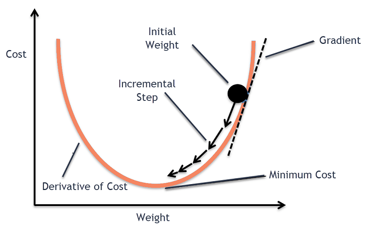
Gradient-based optimization is a well-established and powerful technique for finding the minimum or maximum of a function. Specifically, it leverages the gradient, a vector pointing in the direction of the function's steepest ascent, to guide the iterative optimization process.

Intuition

Consider a function $f(x)$ that you want to minimize. At each $x$, you can compute the derivative, $f'(x)$, which indicates the "slope" or rate of change of the function at $x$. The gradient generalizes this concept to multivariable functions and provides a direction to follow for the most rapid increase or decrease in the function's output.

In the context of machine learning models, the goal is often to minimize a loss function, representing the discrepancy between predicted and actual outputs. By iteratively updating the model's parameters in the opposite direction of the gradient, you can reach a parameter set that minimizes the loss function.

Core Concepts

• Gradient: A vector of partial derivatives with respect to each parameter. For a function $f(x_1, x_2, ..., x_n)$, the gradient is denoted as $\nabla f$.

• Learning Rate: A scalar that controls the step size in the parameter update. Too large values can lead to overshooting the minimum, while too small can slow down convergence.

• Optimization Algorithms: Variations of the basic gradient descent algorithm that offer improvements in computational efficiency or convergence.

• Batch Size: In stochastic gradient descent, the gradient is computed using a subset of the training data. The size of this subset is the batch size.

Code Example: Gradient Descent

Here is the Python code:

import numpy as np

def gradient_descent(x, learning_rate, num_iterations):
    for _ in range(num_iterations):
        grad = compute_gradient(x)
        x -= learning_rate * grad
    return x

def compute_gradient(x):
    return 2 * x  # Example gradient for a quadratic function

# Usage
x_initial = 4
learning_rate = 0.1
num_iterations = 100
x_min = gradient_descent(x_initial, learning_rate, num_iterations)

In this example, the function being optimized is a simple quadratic function, and the gradient is $2x$. The learning rate ($0.1$) dictates the step size, and the number of iterations is set to 100.

4. Why is convexity important in optimization problems?

Convexity in optimization refers to the shape of the objective function. When the function is convex, it is bowl-shaped and characterized by a global minimum, making optimization straightforward.

Core Concepts

• Global Minima: Convex functions have a single global minimum, simplifying the optimization process.
• First-Order Optimality: The global minimum is also a local minimum. Therefore, first-order optimality (gradient descent) ensures convergence to the global minimum.
• Second-Order Optimality: The Hessian matrix is positive semi-definite everywhere for convex functions. This property is utilized in second-order methods, such as Newton's method.
• Unique Solution: Convex functions, if strictly convex, have a unique global minimum. In the case of non-strict convexity, the global minimum remains unique under mild conditions.

Real-World Implications

• Reliable Optimization: Convergence to a global minimum is assured, providing confidence in your optimization results.
• General Practicality: Convexity is a commonly occurring assumption.

Code Example: Convex vs. Non-Convex Functions

Here is the Python code:

import numpy as np
import matplotlib.pyplot as plt

# Convex function: f(x) = x^2
x_convex = np.linspace(-5, 5, 100)
y_convex = x_convex ** 2

# Non-convex function: f(x) = x^4 - 3x^3 + 2
x_non_convex = np.linspace(-1, 3, 100)
y_non_convex = x_non_convex ** 4 - 3 * x_non_convex ** 3 + 2

plt.plot(x_convex, y_convex, label='Convex: $f(x) = x^2$')
plt.plot(x_non_convex, y_non_convex, label='Non-Convex: $f(x) = x^4 - 3x^3 + 2$')
plt.legend()
plt.title('Convex and Non-Convex Functions')
plt.xlabel('x')
plt.ylabel('f(x)')
plt.show()

5. Distinguish between local minima and global minima.

Minimization in the context of machine learning and mathematical optimization refers to finding the minimum of a function. There are different types of minima, such as local minima, global minima, and saddle points.

Defining Minima

• Global Minimum: This is the absolute lowest point in the entire function domain.
• Local Minimum: A point that is lower than all its neighboring points but not necessarily the lowest in the entire function domain.

Challenges in Minima Identification

Minimizing complex, high-dimensional functions can pose several challenges:

• Saddle Points: These are points that satisfy the first-order optimality conditions but are neither minima nor maxima.
• Ridges: Functions can have regions that are nearly flat but not exactly so, making them susceptible to stagnation.
• Plateaus: These are long-lasting regions of uncertain decrease in the function value.

Algorithms and Techniques

Many optimization algorithms attempt to navigate around or through these challenges. For instance, stochastic methods such as stochastic gradient descent and mini-batch gradient descent select only a subset of the data for calculating gradient, which can help navigate saddle points and plateaus.

Avoiding Local Optima

Several advanced techniques help algorithms escape local minima and other sub-optimal points:

• Non-Convex Optimization Methods: These are suited for functions with multiple minima and include genetic algorithms, particle swarm optimization, and simulated annealing.
• Multiple Starts: Ensures that an algorithm runs multiple times from different starting points and selects the best final outcome.
• Adaptive Learning Rate Methods: Algorithms like Adam adjust the learning rate for each parameter, potentially helping navigate non-convex landscapes.

Practical Considerations

When optimizing functions, especially in the context of machine learning models, it's often computationally demanding to find global minima. In practice, the focus shifts from finding the global minimum to locating a sufficiently good local minimum.

This shift is practical because:

• Many real-world problems have local minima that are nearly as good as global minima.
• The potentially high computational cost of finding global minima in high-dimensional spaces might outweigh the small performance gain.

Code Example: Local and Global Minima

Here is the Python code:

import matplotlib.pyplot as plt
import numpy as np

# Define the function
def func(x):
    return 0.1*x**4 - 1.5*x**3 + 6*x**2 + 2*x + 1

# Generate x values
x = np.linspace(-2, 7, 100)
# Generate corresponding y values
y = func(x)

# Plot the function
plt.figure()
plt.plot(x, y, label='Function')
plt.xlabel('x')
plt.ylabel('f(x)')

# Mark minima
minima = np.array([0.77, 3.03, 5.24])
plt.scatter(minima, func(minima), c='r', label='Minima')

plt.legend()
plt.show()

6. What is a hyperparameter, and how does it relate to the optimization process?

In machine learning, hyperparameters are settings that control the learning process and the structure of the model, as opposed to the model's learned parameters (such as weights and biases).

Hyperparameters are key in the optimization process as they affect the model's ability to generalize from the training data to unseen data. They can significantly influence the model's performance, including its speed and accuracy.

Distinction from Model Parameters

• Learned Parameters (Model Weights): These are optimized during the training process by methods like gradient descent to minimize the loss function.

• Hyperparameters: These are set prior to training and guide the learning process. The choices made for hyperparameters influence how the learning process unfolds and, consequently, the model's performance.

Hyperparameter Impact

• Model Complexity: Hyperparameters like the number of layers in a neural network or the depth of a decision tree define the model structure's intricacy.
• Learning Rate: This hyperparameter contributes to the broadness vs. precision of the optimization landscape search, effectively influencing the speed and accuracy of the model optimization.
• Regularization Strength: L1 and L2 regularization hyperparameters in models like logistic regression or neural networks control the degree of overfitting during training.

Validation for Hyperparameters

Given that the optimal set of hyperparameters varies across datasets and even within the same dataset, it is standard practice to investigate different hyperparameter configurations.

This is typically accomplished via a split of the training data: a portion is used for training, while the remaining section, known as the validation set, is employed for hyperparameter tuning. Techniques like cross-validation that repeatedly train the model on various sections of the training dataset can be another option.

The model's performance is evaluated on the validation set using a selected metric, like accuracy or mean squared error. The configuration that achieves the best performance, as per the specific metric, is adopted.

Hyperparameter Tuning Process

The search for the best hyperparameter configuration is formalized often as a hyperparameter tuning problem. It is typically done using automated algorithms or libraries like Grid Search, Random Search, or more advanced methods like Bayesian optimization or in the case of deep learning, genetic algorithms or neural architecture search (NAS).

The selected technique explores through the hyperparameter space according to a defined strategy, like grid exploration, uniform random sampling, or more sophisticated approaches like directing the search based on past trials.

Code Example: Hyperparameter Tuning

Here is the Python code:

from sklearn.model_selection import GridSearchCV
from sklearn.ensemble import RandomForestClassifier
from sklearn.datasets import make_classification
from sklearn.model_selection import train_test_split

# Create a sample dataset
X, y = make_classification(n_samples=1000, n_features=20, random_state=42)

# Split the dataset
X_train, X_test, y_train, y_test = train_test_split(X, y, test_size=0.2, random_state=42)

# Initialize the RandomForest classifier
rf = RandomForestClassifier()

# Set hyperparameters grid to search
hyperparameters = {
    'n_estimators': [100, 300, 500],
    'max_depth': [None, 5, 10, 15],
    'min_samples_split': [2, 5, 10]
}

# Initialize the Grid Search with the hyperparameters and evaluate accuracy using 5-fold cross-validation
grid_search = GridSearchCV(rf, hyperparameters, cv=5, n_jobs=-1, verbose=1, scoring='accuracy')

# Fit the Grid Search to our dataset
grid_search.fit(X_train, y_train)

# Get the best hyperparameters
best_params = grid_search.best_params_

# Use the best hyperparameters to re-train the model
best_rf_model = RandomForestClassifier(**best_params)
best_rf_model.fit(X_train, y_train)

# Assess the model's performance on the test set
test_accuracy = best_rf_model.score(X_test, y_test)

print("Best Hyperparameters:", best_params)
print("Test Accuracy:", test_accuracy)

7. Explain the concept of a learning rate.

The learning rate is a hyperparameter that determines the size of the steps taken during the optimization process. It plays a crucial role in balancing the speed and accuracy of learning in iterative algorithms such as gradient descent.

A higher learning rate results in faster convergence, but it's more likely to cause divergence or oscillations. A lower learning rate is more stable but can be computationally expensive and slow.

Mathematics

In the gradient descent algorithm, the learning rate $\alpha$ scales the direction and magnitude of the update:

$$ \text{New Parameter} = \text{Old Parameter} - \alpha \times \text{Gradient} $$

In more advanced optimization algorithms, such as stochastic gradient descent, the learning rate can be further adapted based on previous updates.

Tuning the Learning Rate

Selecting an appropriate learning rate is crucial for the success of optimization algorithms. It's often tuned through experimentation or by leveraging methods such as learning rate schedules and automatic tuning techniques.

Learning Rate Schedules

A learning rate schedule dynamically adjusts the learning rate during training. Common strategies include:

• Step Decay: Reducing the learning rate at specific intervals or based on a predefined condition.
• Exponential Decay: Gradually decreasing the learning rate after a certain number of iterations or epochs.
• Adaptive Methods: Modern optimization algorithms (e.g., AdaGrad, RMSprop, Adam) adjust the learning rate based on previous updates. These methods effectively act as adaptive learning rate schedules.

Automatic Learning Rate Tuning

Several advanced techniques exist to automate the process of learning rate tuning:

• Grid Search and Random Search: Although not specific to learning rates, these techniques involve systematically or randomly exploring hyperparameter spaces. They can be computationally expensive.
• Bayesian Optimization: This method models the hyperparameter space and uses surrogate models to decide the next set of hyperparameters to evaluate, reducing computational resources.
• Hyperband and SuccessiveHalving: These techniques leverage a combination of random and grid search with a pruning mechanism to allocate resources more efficiently.

Code Example: Learning Rate Schedules

Here is the Python code:

import numpy as np
import matplotlib.pyplot as plt

num_iterations = 100
base_learning_rate = 0.1

# Step Decay
def step_decay(learning_rate, step_size, decay_rate, epoch):
    return learning_rate * decay_rate ** (np.floor(epoch / step_size))

step_sizes = [25, 50, 75]
decay_rate = 0.5

learning_rates = [step_decay(base_learning_rate, step, decay_rate, np.arange(num_iterations)) for step in step_sizes]

# Exponential Decay
def exponential_decay(learning_rate, decay_rate, epoch):
    return learning_rate * decay_rate ** epoch

decay_rate = 0.96
learning_rates_exp = [exponential_decay(base_learning_rate, decay_rate, epoch) for epoch in np.arange(num_iterations)]

plt.plot(np.arange(num_iterations), learning_rates[0], label='Step Decay (Step Size: 25)')
plt.plot(np.arange(num_iterations), learning_rates[1], label='Step Decay (Step Size: 50)')
plt.plot(np.arange(num_iterations), learning_rates[2], label='Step Decay (Step Size: 75)')
plt.plot(np.arange(num_iterations), learning_rates_exp, label='Exponential Decay')
plt.xlabel('Epoch')
plt.ylabel('Learning Rate')
plt.title('Learning Rate Schedules')
plt.legend()
plt.show()

8. Discuss the trade-off between bias and variance in model optimization.

Bias-Variance Trade-Off is a fundamental concept in machine learning that entails balancing two sources of model error: bias and variance.

Bias: Underfitting

• Description: Represents the error introduced by approximating a real-world problem with a simplistic model. High bias often leads to underfitting.
• Impact: The model is overly general, making it unable to capture the complexities in the data.
• Optimization Approach: Increase model complexity by, for example, using non-linearities and more features.

Variance: Overfitting

• Description: Captures the model's sensitivity to fluctuations in the training data. High variance often results in overfitting.
• Impact: The model becomes overly tailored to the training data and fails to generalize well to new, unseen data points.
• Optimization Approach: Regularize the model by, for example, reducing the number of features or adjusting regularization hyperparameters.

Balancing Bias and Variance

Identifying the optimal point between bias and variance is the key to creating a generalizable machine learning model.

Model Complexity

• Low Complexity (High Bias, Low Variance): Results in underfitting. Assumes too much simplicity in the data, causing both training and test errors to be high.

• High Complexity (Low Bias, High Variance): Can lead to overfitting, where the model is tailored too closely to the training data. While this results in a low training error, the test error, and thus the model's generalizability can be high.

Bias-Variance Curve

The relationship between model complexity, bias, and variance is often described using a Bias-Variance curve, which shows the expected test error as a function of model complexity.

Strategies for Bias-Variance Trade-Off

• Cross-Validation: Using methods like k-fold cross-validation helps to better estimate model performance on unseen data, allowing for a more informed model selection.

• Regularization: Techniques like L1 (LASSO) and L2 (ridge) regularization help prevent overfitting by adding a penalty term.

• Feature Selection: Identifying and including only the most relevant features can help combat overfitting, reducing model complexity.

• Ensemble Methods: Combining predictions from multiple models can often lead to reduced variance. Examples include Random Forest and Gradient Boosting.

• Hyperparameter Tuning: Choosing the right set of hyperparameters, such as learning rates or the depth of a decision tree, can help strike a good balance between bias and variance.

Model Evaluation Metrics

• Evaluation Metrics: Metrics such as the accuracy, precision, recall, F1-score, and mean squared error (MSE) are commonly used to gauge model performance.

• Training and Test Error: The use of these errors can help you evaluate where your model stands in such a trade-off.

Visualizing Bias and Variance

You can visualize bias and variance using learning curves and validation curves. These curves plot model performance, often error, as a function of a given hyperparameter, dataset size, or any other relevant measure.

Here is the Python code:

import matplotlib.pyplot as plt
from sklearn.model_selection import learning_curve, validation_curve
from sklearn.tree import DecisionTreeRegressor

# Create a decision tree model
model = DecisionTreeRegressor()

# Calculate learning curves
train_sizes, train_scores, test_scores = learning_curve(model, X, y, train_sizes=np.linspace(0.1, 1.0, 5))
train_scores_mean = np.mean(train_scores, axis=1)
test_scores_mean = np.mean(test_scores, axis=1)

# Plot learning curves
plt.plot(train_sizes, train_scores_mean, 'o-', color="r", label="Training score")
plt.plot(train_sizes, test_scores_mean, 'o-', color="g", label="Cross-validation score")
plt.legend(loc="best")
plt.show()

# Calculate validation curves for a particular hyperparameter (e.g., tree depth)
param_range = np.arange(1, 20)
train_scores, test_scores = validation_curve(model, X, y, param_name="max_depth", param_range=param_range, cv=5)
train_scores_mean = np.mean(train_scores, axis=1)
test_scores_mean = np.mean(test_scores, axis=1)

# Plot validation curve
plt.plot(param_range, train_scores_mean, 'o-', color="r", label="Training score")
plt.plot(param_range, test_scores_mean, 'o-', color="g", label="Cross-validation score")
plt.legend(loc="best")
plt.show()

9. What is Gradient Descent, and how does it work?

Gradient Descent serves as a fundamental optimization algorithm in a plethora of machine learning models. It helps fine-tune model parameters for improved accuracy and builds the backbone for more advanced optimization techniques.

Core Concept

Gradient Descent minimizes a Loss Function by iteratively adjusting model parameters in the opposite direction of the gradient $\nabla$, yielding the steepest decrease in loss:

$$ \theta_{new} = \theta_{old} - \alpha \nabla J(\theta_{old}) $$

Here, $\theta$ represents the model's parameters, $\alpha$ symbolizes the Learning Rate for each iteration, and $J(\theta)$ is the loss function.

Visual Representation

Variants & Use Cases

• Batch Gradient Descent: Updates parameters using the gradient computed from the entire dataset.
• Stochastic Gradient Descent (SGD): Calculates the gradient using one data point at a time, suiting larger datasets and dynamic models.
• Mini-Batch Gradient Descent: Strikes a balance between the previous two techniques by computing the gradient across smaller, random data subsets.

Code Example: Gradient Descent

Here is the Python code:

def gradient_descent(X, y, theta, alpha, num_iters):
    m = len(y)
    for _ in range(num_iters):
        h = np.dot(X, theta)
        loss = h - y
        cost = np.sum(loss**2) / (2 * m)
        gradient = np.dot(X.T, loss) / m
        theta -= alpha * gradient
    return theta

10. Explain Stochastic Gradient Descent (SGD) and its benefits over standard Gradient Descent.

Stochastic Gradient Descent (SGD) is an iterative optimization algorithm known for its computational efficiency, especially with large datasets. It's an extension of the more general Gradient Descent method.

Key Concepts

• Target Function: SGD minimizes an objective (or loss) function, such as a cost function in a machine learning model, using the first-order derivative.
• Iterative Update: The algorithm updates the model's parameters in small steps with the goal of reducing the cost function.
• Stochastic Nature: Instead of using the entire dataset for each update, SGD randomly selects just one data point or a small batch of data points.

Algorithm Steps

1. Initialization: Choose an initial parameter vector.
2. Data Shuffling: Randomly shuffle the dataset to randomize the data point selection in each SGD iteration.
3. Parameter Update: For each mini-batch of data, update the parameters based on the derivative of the cost.
4. Convergence Check: Stop when a termination criterion, such as a maximum number of iterations or a small gradient norm, is met.

$$ \theta_{i+1} = \theta_i - \alpha \nabla{J(\theta_i; x_i, y_i)} $$

• $\alpha$ represents the learning rate, and $J$ is the cost function. $x_i, y_i$ are the input and output corresponding to the selected data point.

Benefits Over GD

• Computational Efficiency: Especially with large datasets, as it computes the gradient on just a small sample.
• Memory Conservation: Due to its mini-batch approach, it's often less memory-intensive than full-batch methods.
• Better Convergence with Noisy Data: Random sampling can aid in escaping local minima and settling closer to the global minimum.
• Faster Initial Progress: Even early iterations might yield valuable updates.

Code Example: SGD in sklearn

Here is the Python code:

from sklearn.linear_model import SGDRegressor
from sklearn.datasets import load_boston
from sklearn.model_selection import train_test_split
from sklearn.preprocessing import StandardScaler
from sklearn.metrics import mean_squared_error
import numpy as np

# Load the data
data = load_boston()
X, y = data.data, data.target

# Data splitting
X_train, X_test, y_train, y_test = train_test_split(X, y, test_size=0.2, random_state=42)

# Feature scaling
scaler = StandardScaler()
X_train = scaler.fit_transform(X_train)
X_test = scaler.transform(X_test)

# Initialize the model
sgd_regressor = SGDRegressor()

# Train the model
sgd_regressor.fit(X_train, y_train)

# Make predictions
y_pred = sgd_regressor.predict(X_test)

# Evaluate the model
mse = mean_squared_error(y_test, y_pred)
print("Mean Squared Error:", mse)

In this example, SGDRegressor from sklearn automates the Stochastic Gradient Descent process for regression tasks.

11. Describe the Momentum method in optimization.

Momentum in optimization techniques is based on the idea of giving the optimization process persistent direction.

In practical terms, this means that steps taken in previous iterations are used to inform the direction of the current step, leading to faster convergence.

Key Concepts

• Memory Effect: By accounting for past gradients, momentum techniques ensure the optimization process is less susceptible to erratic shifts in the immediate gradient direction.

• Inertia and Damping: Momentum introduces "inertia" by gradually accumulating step sizes in the direction of previous gradients. Damping prevents over-amplification of these accumulated steps.

Momentum Equation

The update rule for the momentum method can be mathematically given as:

$$ $$ v_t &= \gamma v_{t-1} + \eta \nabla J(\theta) \\ \theta &= \theta - v_t $$ $$

Where:

• $v_t$ denotes the update at time $t$.

• $\gamma$ represents the momentum coefficient.

• $\eta$ is the learning rate.

• $\nabla J(\theta)$ is the gradient.

• Momentum Coefficient ($\gamma$): This value, typically set between 0.9 and 0.99, determines the extent to which previous gradients influence the current update.

Code Example: Momentum

Here is the Python code:

# Initialize momentum hyperparameter
gamma = 0.9
# Initialize the parameter search space
theta = 0
# Initialize momentum variable
v = 0
# Assign a learning rate
learning_rate = 0.1

# Compute new velocity with momentum
v = gamma * v + learning_rate * gradient
# Update the parameter using the momentum-boosted gradient
theta = theta - v

12. What is the role of second-order methods in optimization, and how do they differ from first-order methods?

Second-order methods, unlike first-order ones, consider curvature information when determining the optimal step size. This often results in better convergence and, with a well-chosen starting point, can lead to faster convergence.

Key Concepts

Hessian Matrix

The Hessian Matrix represents the second-order derivatives of a multivariable function. It holds information about the function's curvature, aiding in identifying valleys and hills.

Mathematically, for a function $f(\mathbf{x})$ with $n$ variables, the Hessian Matrix, $\mathbf{H}$, is defined as:

$$ \mathbf{H}_{ij} = \frac{\partial^2 f(\mathbf{x})}{\partial x_i \partial x_j} $$

Curvature and Convergence

The direction of steepest descent with respect to adaptive metrics offered by the Hessian Matrix can lead to quicker convergence.

Utilizing the Hessian allows for a quadratic approximation of the objective function. Combining the gradient and curvature information yields a more informed assessment of the landscape.

Key Methods

Algorithms that incorporate second-order information include:

• Newton-Raphson Method: Uses the Hessian and gradient to make large, decisive steps.
• Gauss-Newton Method: Tailored for non-linear least squares problems in which precise definitions of the Hessian are unavailable.
• Levenberg-Marquardt Algorithm: Balances the advantages of the Gauss-Newton and Newton-Raphson methods for non-linear least squares optimization.

13. How does the AdaGrad algorithm work, and what problem does it address?

AdaGrad, short for Adaptive Gradient Algorithm, is designed to make smaller updates for frequently occurring features and larger updates for infrequent ones.

Core Mechanism

The key distinction of AdaGrad is that it adapts the learning rate on a per-feature basis. Let $G_{t, i}$ be the cumulative sum of squared gradients for feature $i$ up to step $t$:

$$ G_{t, i} = G_{t-1, i} + g_{t, i}^2 $$

where $g_{t, i}$ is the gradient of feature $i$ at time $t$.

The update rule becomes:

$$ w_{t+1, i} = w_{t, i} - \frac{\eta}{\sqrt{G_{t, i} + \epsilon}} \cdot g_{t, i} $$

Here, $\eta$ denotes the global learning rate and $\epsilon$ prevents division by zero.

Code Example: AdaGrad

Here is the Python code:

import numpy as np

def adagrad_update(w, g, G, lr, eps=1e-8):
    return w - (lr / (np.sqrt(G) + eps)) * g, G + g**2

# Initialize parameters
w = np.zeros(2)
G = np.zeros(2)

# Perform update
lr = 0.1
gradient = np.array([1, 1])
w, G = adagrad_update(w, gradient, G, lr)

print(f'Updated weights: {w}')

Addressing Sparse Data

Incorporating unique features, like rare words in text processing, is one of AdaGrad's strengths. This makes it particularly suitable for non-linear optimization tasks when data is sparse.

Limitations and Variants

While potent, AdaGrad has some shortcomings, such as the continuously decreasing learning rate. This led to the development of extensions like RMSProp and Adam, which offer refined strategies for adaptive learning rates.

14. Can you explain the concept of RMSprop?

RMSprop (Root Mean Square Propagation) is an optimization algorithm designed to manage the learning rate during training. It is especially useful in non-convex settings like training deep neural networks.

At its core, RMSprop is a variant of Stochastic Gradient Descent (SGD) and bears similarities to AdaGrad.

Key Components

• Squaring of Gradients: Dividing the current gradient by the root mean square of past gradients equates to dividing the learning rate by an estimate of the variance which can help in reaching the optimum point more efficiently in certain cases.

• Leaky Integration: The division involves exponential smoothing of the squared gradient, which acts as a leaky integrator to address the problem of vanishing learning rates.

Algorithm Steps

1. Compute the gradient:
   

2. Accumulate squared gradients using a decay rate:

4. Update the parameters using the adjusted learning rate:
   

Here, is the decay rate, usually set close to 1, and is a small smoothing term to prevent division by zero.

Code Example: RMSprop

Here is the Python code:

def rmsprop_update(theta, dtheta, cache, decay_rate=0.9, learning_rate=0.001, epsilon=1e-7):
    cache = decay_rate * cache + (1 - decay_rate) * (dtheta ** 2)
    theta += - learning_rate * dtheta / (np.sqrt(cache) + epsilon)
    return theta, cache

15. Discuss the Adam optimization algorithm and its key features.

Adam (Adaptive Moment Estimation) is an efficient gradient-descent optimization algorithm, combining ideas from both RMSProp (which uses a running average of squared gradients to adapt learning rates for each individual model parameter) and momentum. Adam further incorporates bias correction, enabling faster convergence.

Key Features

• Adaptive Learning Rate: Adam dynamically adjusts learning rates for each parameter, leading to quicker convergence. This adaptiveness is particularly helpful for sparse data and non-stationary objectives.

• Bias Correction: Adam uses bias correction to address the initial time steps' imbalances, enhancing early optimization.

• Momentum: Encouraging consistent gradients, the algorithm utilizes past gradients' exponential moving averages.

• Squaring of Gradients: This underpins the mean square measure in momentum.

Algorithm Overview

Adam computes exponentially weighted averages of gradients and squared gradients, much like RMSProp, and additionally includes momentum updates. These are calculated at each optimization step to determine parameter updates. Let's look at the detailed formulas:

Smoothed Gradients:

Here, and denote the smoothed gradient and the squared smoothed gradient, respectively.

Bias-Corrected Averages:

After bias correction, and represent unbiased estimates of the first moment (the mean) and the second raw moment (the uncentered variance) of the gradients.

Parameter Update:

Where is the learning rate, is a small constant for numerical stability, and denotes model parameters.

Code example: Adam Optimization

Here is the Python code:

import numpy as np

def adam_optimizer(grad, lr=0.001, beta1=0.9, beta2=0.999, eps=1e-8):
    # Initialize internal variables
    m = np.zeros_like(grad)
    v = np.zeros_like(grad)
    t = 0
    
    # Update parameters
    t += 1
    m = beta1 * m + (1 - beta1) * grad
    v = beta2 * v + (1 - beta2) * grad**2
    
    # Bias-corrected averages
    m_hat = m / (1 - beta1**t)
    v_hat = v / (1 - beta2**t)
    
    # Parameter update
    return lr * m_hat / (np.sqrt(v_hat) + eps)

Explore all 50 answers here 👉 Devinterview.io - Optimization