
You can also find all 55 answers here 👉 Devinterview.io - Model Evaluation
Model evaluation in machine learning is the process of determining how well a trained model generalizes to new, unseen data. It helps in selecting the best model for a task, assessing its performance against expectations, and identifying any issues such as overfitting or underfitting.
Predictive performance is measured in classification tasks through metrics such as accuracy, precision, recall, F1 score, and area under the ROC curve (AUC-ROC). For regression, commonly used metrics include mean squared error (MSE), root mean squared error (RMSE), mean absolute error (MAE), and
Overfitting occurs when a model is excessively complex, performing well on training data but poorly on new, unseen data. This is typically identified when there is a significant difference between the performance on the training and test sets. Cross-validation can help offset this.
Underfitting results from a model that is too simple, performing poorly on both training and test data. It can be recognized if even model's performance on the training set is not satisfactory.
- Train-Test Split: Initially, the dataset is divided into separate training and testing sets. The model is trained on the former and then evaluated using the latter to approximate how the model will perform on new data.
from sklearn.model_selection import train_test_split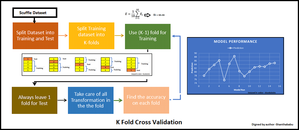
X_train, X_test, y_train, y_test = train_test_split(X, y, test_size=0.2)- k-Fold Cross-Validation: The dataset is divided into k folds (typically 5 or 10), and each fold is used as the test set k-1 times, with the rest as the training set. This is repeated k times, and the results are averaged. It's more reliable than a single train-test split.
from sklearn.model_selection import cross_val_score
scores = cross_val_score(model, X, y, cv=5)-
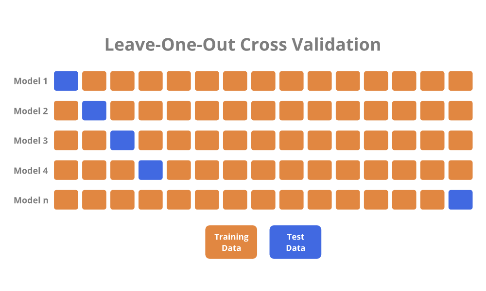
Leave-One-Out Cross-Validation (LOOCV): A more extreme form of k-fold where k is set to the number of data points. It can be computationally expensive but is helpful when there are limited data points.
-
Bootstrapping: A resampling technique where multiple datasets are constructed by sampling with replacement from the original dataset. The model is trained and tested on these bootstrapped datasets, and the average performance is taken as the overall performance estimate.
Jackknife: A specific type of bootstrapping where each dataset is generated by removing one data point.
Each of these is a distinct dataset used for different stages of model training and evaluation. Training Dataset is usually the largest, while Test Dataset is typically a 70-30 or 80-20 split.
A well-divided data ensures better evaluation of the model performance and better generalization of the model on unseen data.
- Training Data: Used by the ML model to optimize its parameters. It's also what the model has "learned" from.
- Validation Data: (Optionally used in training) The model's performance on this set is assessed after each round of training, enabling fine-tuning or early stopping.
- Test Data: This dataset is entirely unseen by the model and is used to evaluate its final, unbiased performance.
- Training Data: The most critical as it is used to fit the model.
- Validation Data: Used to guide training, ensure model isn't overfitting.
- Test Data: The ultimate judge of model performance.
Typically, one trains the model using the training dataset, evaluates it using the validation dataset, adjusts the model (e.g., hyperparameters) until both its training and validation performance are satisfactory, and then finally evaluates the model using the test dataset to check its robustness.
Here is the Python code:
from sklearn.model_selection import train_test_split

# Split data into training and test datasets
X_train, X_test, y_train, y_test = train_test_split(X, y, test_size=0.3, random_state=42)

# Further split training data into training and validation
X_train, X_val, y_train, y_val = train_test_split(X_train, y_train, test_size=0.2, random_state=42)Cross-validation is a widely used technique in machine learning for model evaluation. Instead of relying on a single train-test split, cross-validation uses multiple partitions of the data to build and assess a model.
- Efficient Data Utilization: Each data point is used for both training and validation multiple times, thus maximizing data utilization.
- Reduction in Variability: Averaging performance over multiple validation sets helps minimize the variability in model performance metrics.
- Robustness: Ensures that model evaluation isn't excessively influenced by the specific instances in a single train-test split.
- Model Selection Guidance: By evaluating different models on multiple cross-validation folds, it provides more reliable guidance for model selection.
The dataset is divided into
Python code example using scikit-learn:
from sklearn.model_selection import KFold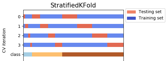
kf = KFold(n_splits=5, shuffle=True, random_state=42)This is helpful when the target classes are imbalanced. It ensures that each fold has a similar distribution of target classes as the whole dataset.
Python code example using scikit-learn:
from sklearn.model_selection import StratifiedKFold
skf = StratifiedKFold(n_splits=5, shuffle=True, random_state=42)In this method, only one individual observation serves as the test set, and the rest acts as the training set.
While LOOCV can be computationally expensive for large datasets, it's virtually bias-free.
Python code example using scikit-learn:
from sklearn.model_selection import LeaveOneOut
loo = LeaveOneOut()To further strengthen the robustness of model assessment, K-Fold is often repeated multiple times, shuffling the data at each repetition.
Python code example using scikit-learn:
from sklearn.model_selection import RepeatedKFold
rkf = RepeatedKFold(n_splits=5, n_repeats=3, random_state=42)Precision, recall, and F1-score are metrics primarily used for evaluating binary classification tasks, though they can be extended to support multi-class problems.
Precision quantifies the number of True Positives (TP) in relation to the total number of positive predictions (True Positives and False Positives, or FP).
It represents the probability that a data point classified as positive is truly positive. High precision means the classifier is very trustworthy when it labels an instance as positive.
Recall, also known as sensitivity or the True Positive Rate (TPR), measures the proportion of actual positives that were correctly identified out of all true positives and false negatives.
Recall captures the extent to which the classifier is able to identify all actual positive instances. High recall indicates that the classifier is effective at finding most of the positive instances.
The F1-score, often referred to as the Harmonic Mean of precision and recall, provides a balance between the two measures.
The F1-score is useful when there is an uneven class distribution. It combines precision and recall into a single metric, making it convenient for scenarios where both are important, such as in medical diagnostic systems.
The Confusion Matrix is a foundational tool in the evaluation of classification algorithms. It provides a comprehensive breakdown of the algorithm's performance and facilitates the calculation of various metrics, such as accuracy, precision, recall, and the F1-score.
A Confusion Matrix for a binary classifier has four primary components:
- True Positives (TP): The number of positive instances correctly classified as positive.
- True Negatives (TN): The number of negative instances correctly classified as negative.
- False Positives (FP): The number of negative instances that are incorrectly classified as positive.
- False Negatives (FN): The number of positive instances that are incorrectly classified as negative.
Here is a visual representation:
| Predicted Negative | Predicted Positive | |
|---|---|---|
| Actual Negative | True Negatives (TN) | False Positives (FP) |
| Actual Positive | False Negatives (FN) | True Positives (TP) |
- Diagonal cells from top-left to bottom-right represent correct classifications.
- Off-diagonal cells represent misclassifications.
The four main metrics derived from the Confusion Matrix are:
Accuracy represents the proportion of correctly classified instances out of the total dataset.
Precision characterizes the proportion of predicted positives that are correct.
Recall captures the proportion of actual positives that are correctly identified.
The F1 score is the harmonic mean of precision and recall, offering a balanced assessment of the classifier's performance.
For multi-class classification, the Confusion Matrix extends to a square matrix with dimensions equal to the number of classes. Each row and column now correspond to a unique class, and the matrix visually summarizes true and false classifications for each class.
For
The sum of each row gives the total number of true instances for the corresponding class, while the sum of the columns provides the total number of instances predicted for each class.
Here is the Python code:
from sklearn.metrics import confusion_matrix, accuracy_score, precision_score, recall_score, f1_score

# Actual classes
y_true = [1, 0, 0, 1, 1, 1, 0, 1, 1, 0]
# Predicted classes
y_pred = [1, 1, 0, 1, 0, 1, 0, 1, 0, 0]

# Computing Confusion Matrix
cm = confusion_matrix(y_true, y_pred)
print("Confusion Matrix:")
print(cm)

# Computing metrics
acc = accuracy_score(y_true, y_pred)
prec = precision_score(y_true, y_pred)
rec = recall_score(y_true, y_pred)
f1 = f1_score(y_true, y_pred)

print(f"Accuracy: {acc:.2f}, Precision: {prec:.2f}, Recall: {rec:.2f}, F1-Score: {f1:.2f}")The ROC (Receiver Operating Characteristic) curve and its numerical counterpart, the Area Under the Curve (AUC), are essential evaluation tools in machine learning, especially for binary classification tasks.
The ROC curve graphically represents the trade-offs between the true positive rate (TPR) and the false positive rate (FPR) at varying classification thresholds.
For instance, choosing a more lenient threshold may increase the true-positive rate, but at the cost of more false positives. By moving this threshold, you can observe the ROC plot "bend" to reflect such changes.

The AUC numerically quantifies the model's ability to distinguish between classes, often interpreted as the likelihood that the classifier will rank a randomly chosen positive instance higher than a randomly chosen negative instance.
A perfect classifier will have an AUC of 1, whereas a random classifier, like one based on a coin toss, has an AUC of 0.5.
The ROC curve is a visual representation of the relationship between the true positive rate and the false positive rate, which are calculated as:
where TP = True Positives, FP = False Positives, TN = True Negatives, and FN = False Negatives.
The AUC is found by computing the area under the ROC curve, typically through numerical integration methods like the trapezoidal rule.
Comparing multiple models using a single metric, such as AUC, can help make quick, high-level performance assessments. Since AUC computes a probability-like measure, it can handle classification thresholds without explicit threshold setting.
-
Baseline: The diagonal line represents a purely random classifier, and any good model should be well above that line.
-
Steepness: The steeper the curve, the better the model. A perfect model would be a vertical line.
-
Shape: The closer to the top-left corner, the better, as this means the model has both high TPR and low FPR across all thresholds.
Here is the Python code:
from sklearn.metrics import roc_curve, roc_auc_score

# Assuming you already have model predictions and ground truth labels
fpr, tpr, thresholds = roc_curve(y_true, y_scores)
auc = roc_auc_score(y_true, y_scores)While accuracy is a popular metric, especially in balanced datasets, it can fall short in certain situations. Here are the reasons:
-
Imbalanced Datasets: When classes are not represented equally, high accuracy can be achieved by simply predicting the majority class. For instance, in a dataste with 95% of examples belonging to class A, a model that predicts class A consistently will still yield 95% accuracy, but it is not useful in reality.
For example, in a medical dataset where only 1% of patients have a rare disease, even a model that labels everyone as negative will still achieve 99% accuracy.
-
Misclassification Costs: Some errors are costlier than others. For instance, in a cancer detection model, a false negative (missing a patient with cancer) is more severe than a false positive (flagging a non-cancer patient for further screening). By only focusing on accuracy, this distinction is lost.
-
Decision Thresholds: In many classification problems, especially those involving probabilities, there is a need to set a threshold for class assignment. Depending on this threshold, a model may vary in terms of true positives, false positives, true negatives, and false negatives. Simply evaluating based on the hard threshold with the best accuracy may not be the best strategy.
To address these limitations, several other metrics exist:
- Precision: This measures the accuracy of positive predictions.
In our cancer example, this is the proportion of correctly identified cancer patients out of all patients labeled as having cancer.
- Recall (Sensitivity): This gauges the model's ability to identify all positives.
For the cancer model, recall is the proportion of correctly identified cancer patients out of all patients who actually have cancer.
- F1 Score: This is the harmonic mean of precision and recall. It provides a balanced view of a model's performance.
For the cancer model, an F1 score gives an overall measure of how well the model is identifying cancer patients while keeping false positives low.
- Area Under the Curve (AUC): This metric is typically used in the context of binary classification. It measures the model's ability to distinguish between positive and negative classes.
-
Business Needs: It is crucial to understand the real-world implications of model decisions. A bank, for instance, may be more concerned with avoiding false negatives in credit risk assessment, whereas false positives in such a scenario are less critical.
-
Regulatory and Ethical Factors: In certain domains, like healthcare, the cost of misclassification can be much higher, demanding models with high precision and recall.
-
Data Characteristics: Instead of a one-size-fits-all approach, models should be evaluated in the context of the data they are applied to.
Let me explain to you what is Overfitting and Underfitting.
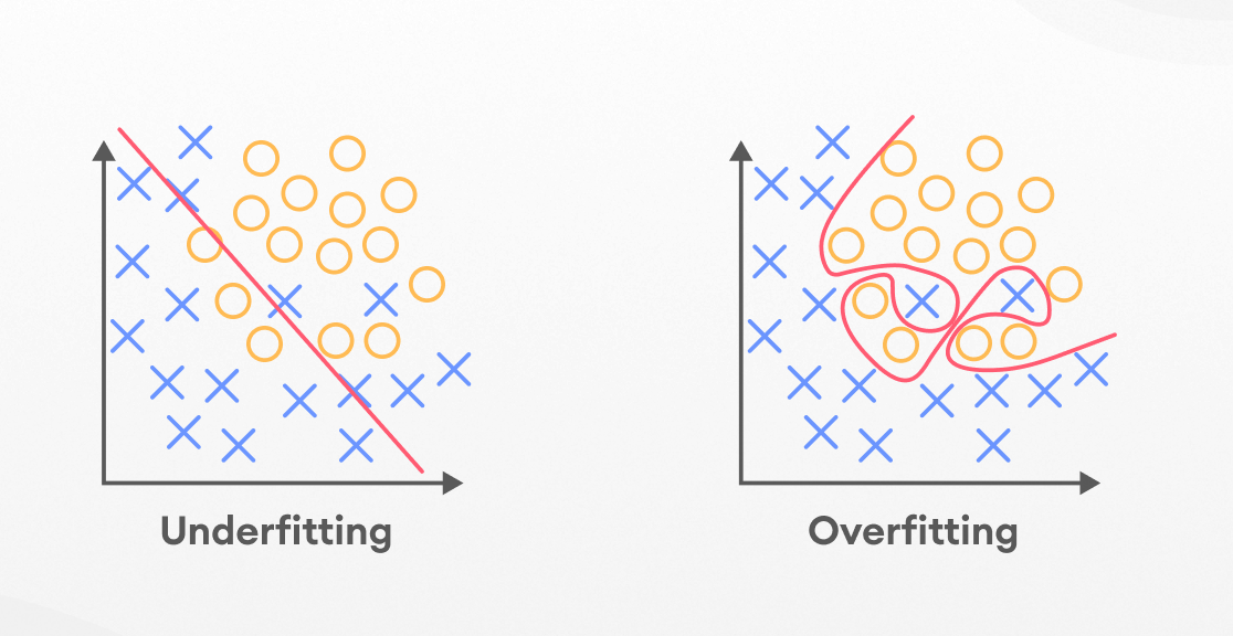
Overfitting occurs when a machine learning model is excessively tailored to idiosyncrasies in the training data, leading to poor generalization on new/unseen data.
Think of it like a student who memorizes past exam answers without truly understanding the subject matter. When faced with new, unseen questions, they'll struggle to answer meaningfully.
In the context of a Decision Tree, overfitting would mean that the tree is too deep, taking into account irrelevant features, and not stopping at a point that would be most beneficial for correct predictions.
- Noisy Data: When training data contain a lot of randomness or errors.
- Feature Overload: Incorporating irrelevant or too many features.
- Inflexible Models: Such as overly complex neural networks or decision trees.
- Lack of Regularization: Failure to include constraints on model parameters.
-
Training vs. Validation Performance: While training data performance might look great, if the model fares significantly worse on validation or test data, it's likely overfit.
-
Learning Curves: Visual representations of accuracy/loss vs. data size can help spot overfitting. A training curve that's improving while the validation curve is deteriorating indicates overfitting.
-
Model Complexity: As you increase the complexity of the model, ideally, the training error should reduce. However, if the validation error starts to increase, that's a sign of overfitting.
-
Cross-Validation: Running a cross-validated performance evaluation can help identify if a model is overfitting.
-
Regularization Tuning: Techniques like L1 or L2 regularization and dropout, when applied mainly to complex models, can assist in controlling overfitting.
-
Feature Selection and Dimensionality Reduction: Utilizing only relevant features or reducing the number of features can also help to address the problem.
-
Ensemble Models: By combining predictions from multiple simpler models, one can often reduce the risk of overfitting.
-
Early Stopping: In settings like neural network training, monitoring validation performance can determine when to halt training to avoid overfitting.
-
Visual Inspection: Sometimes you can tell a model is overfit by just plotting its performance in a clear and informative graph.
Underfitting describes the situation where a machine learning algorithm is too simplistic to capture the underlying structure of the data, leading to poor performance on both the training set and new data.
It's akin to using an overly simplified, high-level summary of a book instead of delving into the details and nuances.
In the context of a decision tree, underfitting would mean that the tree is too shallow and doesn't encapsulate the necessary decision boundaries to make accurate predictions.
- Insufficient Data: The algorithm might not have enough examples to discern patterns accurately.
- Too Simplistic Model: Using a linear model to fit a highly nonlinear dataset is a classic example.
- Inadequate Features: If the algorithm doesn't have enough relevant features to learn from, it's likely to underperform.
-
Low Accuracy Across the Board: Both training and validation accuracies are low, suggesting that the algorithm is unable to capture the underlying patterns.
-
Learning Curves: The accuracy on both training and validation data may stagnate at low levels, indicating underfitting.
-
Model Complexity: Even as you increase the complexity, if both training and validation performance fail to improve, it likely points to underfitting.
-
Cross-Validation: Similar to overfitting, cross-validated performance can give insights into underfitting.
-
Feature Engineering: By improving the set of features that the model learns from, you can often address underfitting.
-
Ensemble Methods: By combining several models, you can often make up for the inadequacies of a single one.
-
Parameter Tuning: For some algorithms, especially those with meta-parameters like "kernel" in SVM, tuning these can sometimes resolve underfitting.
-
Experience: Sometimes, understanding the nature of the problem domain can help identify when a model is underfitting.
Learning curves provide valuable insights into how a model benefits from additional data, offering a practical method for determining the expectations of larger datasets.
Visualizing the relationship between data size and performance helps uncover certain behaviors in a machine learning model:
- Variance and Bias: Indicators such as a large gap between training and validation scores, along with consistently high errors, can signal overfitting.
- Leveling out: If both training and validation errors remain high or show marginal improvement despite increased data, the model might suffer from underfitting.
- Convergence: The convergence of train and validation scores to a low error can highlight a sweet spot for dataset size, beyond which additional data might not yield significant improvements. This is often observed in more complex algorithms or smaller datasets.
Here is the Python code:
import numpy as np
import matplotlib.pyplot as plt
from sklearn.model_selection import learning_curve
from sklearn.linear_model import LogisticRegression

# Generate a mock dataset
X, y = np.arange(100).reshape((50, 2)), np.arange(50)

# Using learning_curve to gather sample sizes and corresponding scores
train_sizes, train_scores, test_scores = learning_curve(LogisticRegression(), X, y, cv=2)

# Calculating mean and variance of scores
train_mean = np.mean(train_scores, axis=1)
train_std = np.std(train_scores, axis=1)
test_mean = np.mean(test_scores, axis=1)
test_std = np.std(test_scores, axis=1)

# Plotting
plt.plot(train_sizes, train_mean, '--', color="#111111", label="Training score")
plt.plot(train_sizes, test_mean, color="#111111", label="Cross-validation score")

plt.fill_between(train_sizes, train_mean - train_std, train_mean + train_std, color="#DDDDDD")
plt.fill_between(train_sizes, test_mean - test_std, test_mean + test_std, color="#DDDDDD")

plt.title("Learning Curve")
plt.xlabel("Training Set Size"), plt.ylabel("Accuracy Score"), plt.legend(loc="best")
plt.tight_layout(), plt.show()Both Explained Variance and R-squared are metrics that provide insights into the performance of a regression model, with a focus on understanding the source and degree of variability in the dependent variable,
Explained Variance is a measure of how well the model captures the variability in the dependent variable,
where:
-
$Y$ is the observed dependent variable. -
$\hat{Y}$ is the predicted dependent variable. -
$\text{Var}$ represents variance.
Advantages:
- Provides a clear understanding of how much variability our model can capture in
$Y$ . - Intuitively straightforward, representing the proportion of variance in
$Y$ that the model captures.
Disadvantages:
- Does not indicate the direction of agreement between observed and predicted values.
- It is sensitive to outliers.
R-squared provides a measure of how well the independent variables (features) explain the variability in the dependent variable,
where:
-
is the sum of squares of residuals, also referred to as unexplained variability.
-
is the total sum of squares, representing the total variability in the dependent variable.
Advantages:
- Provides insights into how much of the variability in the dependent variable is captured by the model.
- Gives a measure that is bounded between 0 and 1, making it easy to interpret and compare across models.
Disadvantages:
- The measure is a bit abstract, not directly giving an intuitive understanding of the proportion of variance explained.
- Can potentially give misleading inferences in some scenarios, especially with multiple regression.
Both R-squared and Explained Variance are widely used, but it's important to use them judiciously in light of their specific strengths and limitations. When assessing model performance, it's often beneficial to use them in conjunction with other metrics to gain a comprehensive understanding.
Regression models are trained to predict continuous numerical values. There are several metrics for evaluating their performance.
-
Mean Absolute Error (MAE):
-
Mean Squared Error (MSE):
-
Root Mean Squared Error (RMSE):
-
$R^2$ Score:
Here is the Python code:
from sklearn.metrics import mean_absolute_error, mean_squared_error, r2_score
import numpy as np

# Generate example data
true_values = np.array([3, -0.5, 2, 7])
predicted_values = np.array([2.5, 0.0, 2, 8])

# Calculate evaluation metrics
mae = mean_absolute_error(true_values, predicted_values)
mse = mean_squared_error(true_values, predicted_values)
rmse = np.sqrt(mse)
r_squared = r2_score(true_values, predicted_values)

# Print results
print(f"Mean Absolute Error (MAE): {mae}")
print(f"Mean Squared Error (MSE): {mse}")
print(f"Root Mean Squared Error (RMSE): {rmse}")
print(f"R-squared (R^2): {r_squared}")When evaluating a classifier, it's crucial to consider a comprehensive suite of performance metrics, tailored to your specific goals and the nature of your data. Commonly employed metrics include:
- Accuracy:
While simple to understand, it can be misleading in imbalanced datasets.
- Precision:
Precision indicates the proportion of true positive predictions among positive predictions made. It's relevant when the cost of false positives is high.
- Recall (Sensitivity):
This metric focuses on the proportion of actual positive instances that were correctly identified. It's useful when the cost of false negatives is high.
- F1 Score:
The F1 Score provides a balanced measure between Precision and Recall.
- Specificity:
It assesses a model's ability to identify negative instances correctly.
- Area under the ROC Curve (AUC-ROC):
ROC curves plot the True Positive Rate (TPR) against the False Positive Rate (FPR) at various threshold settings. The AUC-ROC, or simply AUC, provides a single number to summarize the classifier's performance. An AUC close to 1 indicates the model's strong ability to distinguish between positive and negative classes.
- Area under the Precision-Recall Curve (AUC-PR):
The AUC-PR is a useful metric for imbalanced datasets. It computes the area under the precision-recall curve. A higher value indicates better classifier performance.
- Confusion Matrix:
The confusion matrix provides a detailed breakdown of the model's correct and incorrect predictions, including True Positives (TP), True Negatives (TN), False Positives (FP), and False Negatives (FN).
- Matthews Correlation Coefficient (MCC):
MCC is considered more robust in assessing classifier performance on imbalanced datasets.
- Other Metrics for Probabilistic Classifiers:
- Expected Cost: Incorporates the misclassification cost into the model evaluation.
- Brier Score: Evaluates the accuracy of the predicted probabilities.
The Mean Squared Error (MSE) is a widely-used metric for evaluating the performance of regression models by quantifying the average squared differences between actual and predicted values.
The MSE is calculated as the mean of the squared differences between actual (
- Consistency: Squaring the errors provides a consistent measure, treating both overestimates and underestimates the same way.
- Analytical Convenience: Squaring eliminates cancellations that occur when errors are summed, making differentiability possible.
- Barometer for Variability: Larger errors are magnified, providing a clearer understanding of model performance.
-
Sensitivity to Outliers: Due to squaring, the MSE is greatly influenced by outliers, as even a single large error term can significantly increase the overall value.
-
Scale-Dependence: Metrics such as the
$R^2$ coefficient can help put the MSE value into perspective by providing a percentage measure of variance explained. However, adjusting features to similar scales (via standardization or normalization) can mitigate scale-related issues.
The Area Under the Precision-Recall Curve (AUPRC) provides a nuanced view of classifier performance, useful in settings where class imbalance or varying misclassification costs are present. AUPRC can be especially beneficial in applications where recall or precision are more relevant than a balanced accuracy metric.
The AUPRC is calculated by taking the area under the precision-recall curve. This is usually done using numerical integration techniques, such as the trapezoidal rule.
Unlike the Area Under the Receiver Operating Characteristic curve (AUROC), the AUPRC isn't substantially affected by imbalanced datasets. This makes it a more reliable metric in settings with rare events or skewed class distributions.
AUPRC is particularly well-suited for problems where the positive class is of primary interest. This ensures that the metric is directly attuned to the class that can have more serious consequences, such as disease detection.
-
Medical Diagnosis: In scenarios such as cancer detection, where the focus is on identifying the actual positive cases (cancer patients) accurately, AUPRC provides a more direct assessment compared to AUROC.
-
Anomaly Detection: For systems where the goal is to identify rare or unusual events (like network intrusions, for instance), AUPRC is more relevant as it takes into account the relative rarity of the positive class when assessing model performance.
-
Text Classification with Imbalanced Classes: If a text classifier is built to detect spam, where the positive class (spam) is rarer, AUPRC would be a better choice for evaluating the model's performance, especially compared to a more general metric like accuracy which can be biased.
-
Search Engine Ranking: In this context, the goal would be to rank relevant documents higher. Precision, which is a core component of AUPRC, measures the relevancy better, making AUPRC ideal for this kind of problem.
When evaluating multi-class classification models, you can employ micro-averaging or macro-averaging to consolidate individual class metrics into a single overall performance measure.
Use the micro-average when all classes contribute equally to the evaluation or when instances distribution across classes is imbalanced.
Here's the step-by-step computation of micro-averaged precision:
- True Positives Sum: Count the total true positives for all classes.
- False Positives Sum: Count the total false positives for all classes.
- Precision:
- Recall follows the same computations.
-
$F1$ Score: Harmonic mean of precision and recall.
Use macro-average when it is important to consider per-class performance, especially for class-imbalanced datasets, and when you want to see the model's performance across classes.
- Precision for Each Class:
- Recall for Each Class:
-
$F1$ Score for Each Class:
-
Averaging Metrics: Compute the average values of precision, recall, and
$F1$ score across all classes.
While micro-averaging treats all instances and classes equally, making it less suitable for skewed class distributions, macro-averaging considers each class's performance separately and might be influenced by the representation of majority classes.
So, the best approach often depends on the specific characteristics of the dataset and the evaluation objectives. Sometimes, it is useful to utilize both methods to get a comprehensive understanding of the model's performance.
Explore all 55 answers here 👉 Devinterview.io - Model Evaluation