70 Core Linear Algebra Interview Questions

You can also find all 70 answers here 👉 Devinterview.io - Linear Algebra

1. What is a vector and how is it used in machine learning?

In machine learning, vectors are essential for representing diverse types of data, including numerical, categorical, and text data.

They form the framework for fundamental operations like adding and multiplying with a scalar.

What is a Vector?

A vector is a tuple of one or more values, known as its components. Each component can be a number, category, or more abstract entities. In machine learning, vectors are commonly represented as one-dimensional arrays.

Types of Vectors

• Row Vector: Will have only one row.
• Column Vector: Comprising of only one column.

Play and experiment with the code to know about vectors. Here is the Python code:

# Define a row vector with 3 components
row_vector = [1, 2, 3]

# Define a column vector with 3 components
column_vector = [[1],
                 [2],
                 [3]]

# Print the vectors
print("Row Vector:", row_vector)
print("Column Vector:", column_vector)

Common Vector Operations in Machine Learning

Addition

Each corresponding element is added.

$$ \begin{bmatrix} 1 \\ 2 \\ 3 \end{bmatrix} + \begin{bmatrix} 4 \\ 5 \\ 6 \end{bmatrix} = \begin{bmatrix} 5 \\ 7 \\ 9 \end{bmatrix} $$

Dot Product

Sum of the products of corresponding elements.

$$ [ \begin{bmatrix} 1 & 2 & 3 \end{bmatrix} \cdot \begin{bmatrix} 4 \\ 5 \\ 6 \end{bmatrix} = 1 \times 4 + 2 \times 5 + 3 \times 6 = 32 ] $$

Multiplying with a Scalar

Each element is multiplied by the scalar.

$$ 2 \times \begin{bmatrix} 1 \\ 2 \\ 3 \end{bmatrix} = \begin{bmatrix} 2 \\ 4 \\ 6 \end{bmatrix} $$

Length (Magnitude)

Euclidean distance is calculated by finding the square root of the sum of squares of individual elements.

$$ | \begin{bmatrix} 1 \\ 2 \\ 3 \end{bmatrix} | = \sqrt{1^2 + 2^2 + 3^2} = \sqrt{14} $$

2. Explain the difference between a scalar and a vector.

Scalars are single, real numbers that are often used as the coefficients in linear algebra equations.

Vectors, on the other hand, are multi-dimensional objects that not only have a magnitude but also a specific direction in a coordinate space. In machine learning, vectors are commonly used to represent observations or features of the data, such as datasets, measurements, or even the coefficients of a linear model.

Key Distinctions

Dimensionality

• Scalar: Represents a single point in space and has no direction.

• Vector: Defines a direction and magnitude in a multi-dimensional space.

Components

• Scalar: Is standalone and does not have components. Scalars can be considered as 0-D vectors.

• Vector: Consists of elements called components, which correspond to the magnitudes of the vector in each coordinate direction.

Mathematical Formulation

• Scalar: Denoted by a lower-case italicized letter

• Vector: Typically represented using a lowercase bold letter (e.g., ) or with an arrow over the variable ( ). Its components can be expressed in a column matrix or as a transposed row vector.

Visualization in 3D Space

• Scalar: Represents a single point with no spatial extent and thus is dimensionless.

• Vector: Extends from the origin to a specific point in 3D space, effectively defining a directed line segment.

3. What is a matrix and why is it central to linear algebra?

At the heart of Linear Algebra lies the concept of matrices, which serve as a compact, efficient way to represent and manipulate linear transformations.

Essential Matrix Operations

• Addition and Subtraction: Dually to arithmetic, matrix addition and subtraction are performed component-wise.

• Scalar Multiplication: Each element in the matrix is multiplied by the scalar.

• Matrix Multiplication: Denoted as $C = AB$, where $A$ is $m \times n$ and $B$ is $n \times p$, the dot product of rows of $A$ and columns of $B$ provides the elements of the $m \times p$ matrix $C$.

• Transpose: This operation flips the matrix over its main diagonal, essentially turning its rows into columns.

• Inverse: For a square matrix $A$, if there exists a matrix $B$ such that $AB = BA = I$, then $B$ is the inverse of $A$.

Two Perspectives on Operations

1. Machine Perspective: Matrices are seen as a sequence of transformations, with emphasis on matrix multiplication. This viewpoint is prevalent in Computer Graphics and other fields.

2. Data Perspective: Vectors comprise the individual components of a system. Here, matrices are considered a mechanism to parameterize how the vectors change.

Visual Representation

• The Cartesian Coordinate System can visually represent transformations through matrices. For example:

• For Reflection: The 2D matrix

flips the y-component.

• For Rotation: The 2D matrix

rotates points by

radians.

• For Scaling: The 2D matrix

scales points by a factor of

in both dimensions.

Application in Multiple domains

Computer Science

• Graphic Systems: Matrices are employed to convert vertices from model to world space and to perform perspective projection.

• Data Science: Principal Component Analysis (PCA) inherently entails eigendecompositions of covariance matrices.

Physics

• Quantum Mechanics: Operators (like Hamiltonians) associated with physical observables are represented as matrices.

• Classical Mechanics: Systems of linear equations describe atmospheric pressure, fluid dynamics, and more.

Engineering

• Control Systems: Transmitting electrical signals or managing mechanical loads can be modeled using state-space or transfer function representations, which rely on matrices.

• Optimization: The notorious Least Squares method resolves linear systems, often depicted as matrix equations.

Business and Economics

• Markov Chains: Navigating outcomes subject to variables like customer choice or stock performance benefits from matrix manipulations.

Textiles and Animation

• Rotoscoping: In earlier hand-drawn animations or even in modern CGI, matrices facilitate transformations and movements of characters or objects.

4. Explain the concept of a tensor in the context of machine learning.

In Machine Learning, a tensor is a generalization of scalars, vectors, and matrices to higher dimensions. It is the primary data structure you'll work with across frameworks like TensorFlow, PyTorch, and Keras.

Tensor Basics

• Scalar: A single number, often a real or complex value.

• Vector: Ordered array of numbers, representing a direction in space. Vectors in $\mathbb{R}^n$ are n-dimensional.

• Matrix: A 2D grid of numbers representing linear transformations and relationships between vectors.

• Higher-Dimensional Tensors: Generalize beyond 1D (vectors) and 2D (matrices) and are crucial in deep learning for handling multi-dimensional structured data.

Key Features of Tensors

• Data Representation: Tensors conveniently represent multi-dimensional data, such as time series, text sequences, and images.
• Flexibility in Operations: Can undergo various algebraic operations such as addition, multiplication, and more, thanks to their defined shape and type.
• Memory Management: Modern frameworks manage underlying memory, facilitating computational efficiency.
• Speed and Parallel Processing: Tensors enable computations to be accelerated through hardware optimizations like GPU and TPU.

Code Example: Tensors in TensorFlow

Here is the Python code:

import tensorflow as tf

# Creating Scalars, Vectors, and Matrices
scalar = tf.constant(3)
vector = tf.constant([1, 2, 3])
matrix = tf.constant([[1, 2], [3, 4]])

# Accessing shapes of the created objects
print(scalar.shape)  # Outputs: ()
print(vector.shape)  # Outputs: (3,)
print(matrix.shape)  # Outputs: (2, 2)

# Element-wise operations
double_vector = vector * 2  # tf.constant([2, 4, 6])

# Reshaping
reshaped_matrix = tf.reshape(matrix, shape=(1, 4))

Real-world Data Use-Cases

• Time-Series Data: Capture events at distinct time points.
• Text Sequences: Model relationships in sentences or documents.
• Images: Store and process pixel values in 2D arrays.
• Videos and Beyond: Handle multi-dimensional data such as video frames.

Beyond deep learning, tensors find applications in physics, engineering, and other computational fields due to their ability to represent complex, multi-dimensional phenomena.

5. How do you perform matrix addition and subtraction?

Matrix addition is an operations between two matrices which both are of the same order $(m \times n)$. The result is a matrix of the same order where the corresponding elements of the two input matrices are added.

Algebraic Representation

Given two matrices:

$$ A= \begin{bmatrix} a_{11} & a_{12} & \ldots & a_{1n} \\ a_{21} & a_{22} & \ldots & a_{2n} \\ \vdots & \vdots & \ddots & \vdots \\ a_{m1} & a_{m2} & \ldots & a_{mn} \end{bmatrix} $$

and

$$ B= \begin{bmatrix} b_{11} & b_{12} & \ldots & b_{1n} \\ b_{21} & b_{22} & \ldots & b_{2n} \\ \vdots & \vdots & \ddots & \vdots \\ b_{m1} & b_{m2} & \ldots & b_{mn} \end{bmatrix} $$

The sum of $A$ and $B$ which is denoted as $A + B$ will be:

$$ A + B = \begin{bmatrix} a_{11} + b_{11} & a_{12} + b_{12} & \ldots & a_{1n} + b_{1n} \\ a_{21} + b_{21} & a_{22} + b_{22} & \ldots & a_{2n} + b_{2n} \\ \vdots & \vdots & \ddots & \vdots \\ a_{m1} + b_{m1} & a_{m2} + b_{m2} & \ldots & a_{mn} + b_{mn} \end{bmatrix} $$

For the projection of these operations in code, you could use Python:

import numpy as np

A = np.array([[1, 2, 3], [4, 5, 6]])
B = np.array([[7, 8, 9], [10, 11, 12]])

result = A + B

6. What are the properties of matrix multiplication?

Matrix multiplication is characterized by several fundamental properties, each playing a role in the practical application of both linear algebra and machine learning.

Core Properties

Closure

The product $AB$ of matrices $A$ and $B$ is a valid matrix, subject to a defined number of columns in $A$ matching the number of rows in $B$.

$$ \begin{aligned} A & : m \times n \\ B & : n \times p \\ AB & : m \times p \end{aligned} $$

Associativity

Matrix multiplication is associative, meaning that the order of multiplication remains consistent despite bracketing changes:

$$ A(BC) = (AB)C $$

Non-Commutativity

In general, matrix multiplication is not commutative:

$$ AB \neq BA $$

This implies that, for matrices to be commutative, they must be square and diagonal.

Distributivity

Matrix multiplication distributes across addition and subtraction:

$$ A(B \pm C) = AB \pm AC $$

Additional Properties

Identity Matrix

When a matrix is multiplied by an identity matrix $I$, the original matrix is obtained:

$$ AI = A $$

Zero Matrix

Multiplying any matrix by a zero matrix results in a zero matrix:

$$ 0 \times A = 0 $$

Inverse Matrix

Assuming that an inverse exists, $AA^{-1} = A^{-1}A = I$. However, not all matrices have multiplicative inverses, and care must be taken to compute them.

Transpose

For a product of matrices $(AB)^T$, the order is reversed:

$$ (AB)^T = B^TA^T $$

7. Define the transpose of a matrix.

The transpose of a matrix is generated by swapping its rows and columns. For any matrix $\mathbf{A}$ with elements $a_{ij}$, the transpose is denoted as $\mathbf{A}^T$ and its elements are $a_{ji}$. In other words, if matrix $\mathbf{A}$ has dimensions $m \times n$, the transpose $\mathbf{A}^T$ will have dimensions $n \times m$.

Transposition Properties

• Self-Inverse: $(\mathbf{A}^T)^T = \mathbf{A}$
• Operation Consistency:
  • For a constant $c$: $(c \mathbf{A})^T = c \mathbf{A}^T$
  • For two conformable matrices $\mathbf{A}$ and $\mathbf{B}$: $(\mathbf{A} + \mathbf{B})^T = \mathbf{A}^T + \mathbf{B}^T$

Code Example: Matrix Transposition

Here is the Python code:

import numpy as np

# Create a sample matrix
A = np.array([[1, 2, 3], [4, 5, 6]])
print("Original Matrix A:\n", A)

# Transpose the matrix using NumPy
A_transpose = np.transpose(A)  # or A.T
print("Transpose of A:\n", A_transpose)

8. Explain the dot product of two vectors and its significance in machine learning.

In machine learning, the dot product has numerous applications from basic data transformations to sophisticated algorithms like PCA and neural networks.

Visual Representation

The dot product $\mathbf{a} \cdot \mathbf{b}$ measures how far one vector $\mathbf{a}$ "reaches" in the direction of another $\mathbf{b}$.

Notable Matrix and Vector Operations Derived From Dot Product

Norm

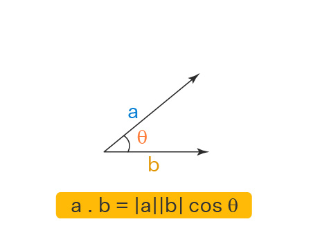
The norm or magnitude of a vector can be obtained from the dot product using:

$$ \lVert \mathbf{a} \rVert = \sqrt{\mathbf{a} \cdot \mathbf{a}} $$

This forms the basis for Euclidean distance and algorithms such as k-nearest neighbors.

Angle Between Vectors

The angle $\theta$ between two non-zero vectors $\mathbf{a}$ and $\mathbf{b}$ is given by:

$$ \cos \theta = \frac{\mathbf{a} \cdot \mathbf{b}}{\lVert \mathbf{a} \rVert \lVert \mathbf{b} \rVert} $$

Projections

The dot product is crucial for determining the projection of one vector onto another. It's used in tasks like feature extraction in PCA and in calculating gradient descent steps in optimization algorithms.

Code Example: Computing the Dot Product

Here is the Python code:

import numpy as np

a = np.array([1, 2, 3])
b = np.array([4, 5, 6])

dot_product = np.dot(a, b)
print("Dot Product:", dot_product)

# Alternatively, you can use the @ operator in recent versions of Python (3.5+)
dot_product_alt = a @ b
print("Dot Product (Alt):", dot_product_alt)

9. What is the cross product of vectors and when is it used?

The cross product is a well-known operation between two vectors in three-dimensional space. It results in a third vector that's orthogonal to both input vectors. The cross product is extensively used within various domains, including physics and computer graphics.

Cross Product Formula

For two three-dimensional vectors and , their cross product is calculated as:

$$ \mathbf{c} = \mathbf{a} \times \mathbf{b} = \begin{bmatrix} a_2b_3 - a_3b_2 \\ a_3b_1 - a_1b_3 \\ a_1b_2 - a_2b_1 \end{bmatrix} $$

Key Operational Properties

• Direction: The cross product yields a vector that's mutually perpendicular to both input vectors. The direction, as given by the right-hand rule, indicates whether the resulting vector points "up" or "down" relative to the plane formed by the input vectors.

• Magnitude: The magnitude of the cross product, denoted by $\lvert \mathbf{a} \times \mathbf{b} \rvert$, is the area of the parallelogram formed by the two input vectors.

Applications

The cross product is fundamental in many areas, including:

• Physics: It's used to determine torque, magnetic moments, and angular momentum.
• Engineering: It's essential in mechanics, fluid dynamics, and electric circuits.
• Computer Graphics: For tasks like calculating surface normals and implementing numerous 3D manipulations.
• Geography: It's utilized, alongside the dot product, for various mapping and navigational applications.

10. How do you calculate the norm of a vector and what does it represent?

The vector norm quantifies the length or size of a vector. It's a fundamental concept in linear algebra, and has many applications in machine learning, optimization, and more.

The most common norm is the Euclidean norm or L2 norm, denoted as $\lVert \mathbf{x} \rVert_2$. The general formula for the Euclidean norm in $n$-dimensions is:

$$ \lVert \mathbf{x} \rVert = \sqrt{x_1^2 + x_2^2 + \ldots + x_n^2} $$

Code Example: Euclidean Norm

Here is the Python code:

import numpy as np

vector = np.array([3, 4])
euclidean_norm = np.linalg.norm(vector)

print("Euclidean Norm:", euclidean_norm)

Other Common Vector Norms

1. L1 Norm (Manhattan Norm): The sum of the absolute values of each component.

$\lVert \mathbf{x} \rVert_1 = |x_1| + |x_2| + \ldots + |x_n|$

2. L-Infinity Norm (Maximum Norm): The maximum absolute component value.

$\lVert \mathbf{x} \rVert_{\infty} = \max_i |x_i|$

3. L0 Pseudonorm: Represents the count of nonzero elements in the vector.

Code Example: Computing L1 and L-Infinity Norms

Here is the Python code:

L1_norm = np.linalg.norm(vector, 1)
L_infinity_norm = np.linalg.norm(vector, np.inf)

print("L1 Norm:", L1_norm)
print("L-Infinity Norm:", L_infinity_norm)

It is worth to note that L2 is suitable for many mathematical operations like inner products and projections, that is why it is widely used in ML.

11. Define the concept of orthogonality in linear algebra.

In linear algebra, vectors in a space can be defined by their direction and magnitude. Orthogonal vectors play a significant role in this framework, as they are perpendicular to one another.

Orthogonality in Euclidean Space

In a real vector space, two vectors $\mathbf{v}$ and $\mathbf{w}$ are orthogonal if their dot product (also known as inner product) is zero:

$$ \mathbf{v} \cdot \mathbf{w} = 0 $$

This defines a geometric relationship between vectors as their dot product measures the projection of one vector onto the other.

General Orthogonality Criteria

For any two vectors $\mathbf{v}$ and $\mathbf{w}$ in an inner product space, they are orthogonal if and only if:

$$ | \mathbf{v} + \mathbf{w} |^2 = | \mathbf{v} |^2 + | \mathbf{w} |^2 $$

This relationship embodies the Pythagorean theorem: the sum of squares of the side lengths of a right-angled triangle is equal to the square of the length of the hypotenuse.

In terms of the dot product, this can be expressed as:

$$ \mathbf{v} \cdot \mathbf{w} = -\frac{1}{2} (|\mathbf{v}|^2 + |\mathbf{w}|^2 - |\mathbf{v} - \mathbf{w}|^2 ) $$

or

$$ \mathbf{v} \cdot \mathbf{w} + \mathbf{v} \cdot (\mathbf{v} - \mathbf{w}) + |\mathbf{v} - \mathbf{w}|^2 - |\mathbf{v}|^2 - |\mathbf{w}|^2 = 0 $$

Practical Applications

1. Geometry: Orthogonality defines perpendicularity in geometry.

2. Machine Learning: Orthogonal matrices are used in techniques like Principal Component Analysis (PCA) for dimensionality reduction and in whitening operations, which ensure zero covariances between variables.

3. Signal Processing: In digital filters and Fast Fourier Transforms (FFTs), orthogonal functions are used because their dot products are zero, making their projections independent.

Code Example: Checking Orthogonality of Two Vectors

Here is the Python code:

import numpy as np

# Initialize two vectors
v = np.array([3, 4])
w = np.array([-4, 3])

# Check orthogonality
if np.dot(v, w) == 0:
    print("Vectors are orthogonal!")
else:
    print("Vectors are not orthogonal.")

12. What is the determinant of a matrix and what information does it provide?

The determinant of a matrix, denoted by $\text{det}(A)$ or $|A|$, is a scalar value that provides important geometric and algebraic information about the matrix. For a square matrix $A$ of size $n \times n$, the determinant is defined.

Core Properties

The determinant of a matrix possesses several key properties:

• Linearity: It's linear in each row and column when the rest are fixed.
• Factor Out: It's factored out if two rows (or columns) are added or subtracted, or a scalar is multiplied to a row (or column).

Calculation Methods

The Laplace expansion method and using the Eigendecomposition of matrices are two common approaches for computing the determinant.

Laplace Expansion

The determinant of a matrix $A$ can be calculated using the Laplace expansion with any row or any column:

$$ \text{det}(A) = \sum_{i=1}^{n} (-1)^{i+j} \cdot a_{ij} \cdot M_{ij} $$

Where $M_{ij}$ is the minor matrix obtained by removing the $i$-th row and $j$-th column, and $a_{ij}$ is the element of matrix $A$ at the $i$-th row and $j$-th column.

Using Eigendecomposition

If matrix $A$ has $n$ linearly independent eigenvectors, $\text{det}(A)$ can be calculated as the product of its eigenvalues.

$$ \text{det}(A) = \prod_{i=1}^{n} \lambda_i $$

Where $\lambda_i$ are the eigenvalues of the matrix.

Geometrical and Physical Interpretations

1. Orientation of Linear Transformations: The determinant of the matrix representation of a linear transformation indicates whether the transformation is orientation-preserving (positive determinant) or orientation-reversing (negative determinant), or if it is just a translation or a projection (determinant of zero).

2. Volume Scaling: The absolute value of the determinant represents the factor by which volumes are scaled when a linear transformation is applied. A determinant of 1 signifies no change in volume, while a determinant of 0 indicates a transformation that collapses the volume to zero.

3. Linear Independence and Invertibility: The existence of linearly independent rows or columns is captured by a non-zero determinant. If the determinant is zero, the matrix is singular and not invertible.

4. Conditioning in Optimization Problems: The determinant of the Hessian matrix, which is the matrix of second-order partial derivatives in optimization problems, provides insights into the local behavior of the objective function, helping to diagnose convergence issues and the geometry of the cost landscape.

Code Example: Computing Determinant

Here is the Python code:

import numpy as np

# Create a random matrix
A = np.random.rand(3, 3)

# Compute the determinant
det_A = np.linalg.det(A)

13. Can you explain what an eigenvector and eigenvalue are?

Eigenvectors and Eigenvalues have paramount significance in linear algebra and are fundamental to numerous algorithms, especially in fields like data science, physics, and engineering.

Key Concepts

• Eigenvalue: A scalar (represented by the Greek letter $\lambda$) that indicates how the corresponding eigenvector is scaled by a linear transformation.

• Eigenvector: A non-zero vector (denoted as $v$) that remains in the same span or direction during a linear transformation, except for a potential scaling factor indicated by its associated eigenvalue.

Math Definition

Let $A$ be a square matrix. A non-zero vector $v$ is an eigenvector of $A$ if $Av$ is a scalar multiple of $v$.

More formally, for some scalar $\lambda$, the following equation holds:

$$ Av = \lambda v $$

In this context, $\lambda$ is the eigenvalue. A matrix can have one or more eigenvalues and their corresponding eigenvectors.

Geometric Interpretation

For a geometric perspective, consider a matrix $A$ as a linear transformation on the 2D space $\mathbb{R}^2$.

• The eigenvectors of $A$ are unchanged in direction, except for potential scaling.
• The eigenvalues determine the scaling factor.

In 3D or higher-dimensional spaces, the eigenvector description remains analogous.

Code Example: Calculating Eigenvalues and Eigenvectors

Here is the Python code:

import numpy as np
# Define the matrix
A = np.array([[2, 1], [1, 3]])
# Calculate eigenvalues and eigenvectors
eigenvalues, eigenvectors = np.linalg.eig(A)
print("Eigenvalues:", eigenvalues)
print("Eigenvectors:", eigenvectors)

Utility in Machine Learning

• Principal Component Analysis (PCA): Eigenvalues and eigenvectors are pivotal for computing principal components, a technique used for feature reduction.
• Data Normalization: Eigenvectors provide directions along which data varies the most, influencing the choice of axes for normalization.
• Singular Value Decomposition (SVD): The guiding principle in SVD is akin to that in eigen-decomposition.

14. How is the trace of a matrix defined and what is its relevance?

The trace of a square matrix, often denoted as $\text{tr}(\mathbf{A})$, is the sum of its diagonal elements. In mathematical notation:

$$ \text{tr}(\mathbf{A}) = \sum_{i=1}^{n} A_{ii} $$

Properties of Trace

• Linearity: For matrices $\mathbf{A}, \mathbf{B},$ and scalar $k$, $\text{tr}(k \mathbf{A}) = k \text{tr}(\mathbf{A})$ and $\text{tr}(\mathbf{A} + \mathbf{B}) = \text{tr}(\mathbf{A}) + \text{tr}(\mathbf{B})$.

• Cyclic Invariance: The trace of $\mathbf{A} \mathbf{B} \mathbf{C}$ is equal to the trace of $\mathbf{B} \mathbf{C} \mathbf{A}$.

• Transposition Invariance: The trace of a matrix is invariant under its transpose: $\text{tr}(\mathbf{A}) = \text{tr}(\mathbf{A}^T)$.

• Trace and Determinant: The trace of a matrix is related to its determinant via characteristic polynomials.

• Trace and Eigenvalues: The trace is the sum of the eigenvalues. This can be shown by putting the matrix in Jordan form where the diagonal elements are the eigenvalues.

• Orthogonal Matrices: For an orthogonal matrix, $\text{tr}(\mathbf{S})$ equals the dimension of the matrix and $\det(\mathbf{S})$ takes the values $\pm 1$.

15. What is a diagonal matrix and how is it used in linear algebra?

A diagonal matrix is a structured linear operator seen in both applied and theoretical linear algebra. In this matrix, non-diagonal elements, which reside off the principal diagonal, are all zero.

Mathematical Representation

A diagonal matrix $D$ is characterized by:

$$ \begin{bmatrix} d_1 & 0 & \cdots & 0 \\ 0 & d_2 & \cdots & 0 \\ \vdots & \vdots & \ddots & \vdots \\ 0 & 0 & \cdots & d_n \end{bmatrix} $$

where $d_1, \ldots, d_n$ are the diagonal entries.

Matrix Multiplication Shortcut

When a matrix is diagonal, matrix multiplication simplifies:

$$ Dx = y $$

can be rewritten as:

$$ \begin{bmatrix} d_1x_1 \\ d_2x_2 \\ \vdots \\ d_nx_n \end{bmatrix} = \begin{bmatrix} y_1 \\ y_2 \\ \vdots \\ y_n \end{bmatrix} $$

This reduces to:

$$ \begin{bmatrix} d_1 & 0 & \cdots & 0 \\ 0 & d_2 & \cdots & 0 \\ \vdots & \vdots & \ddots & \vdots \\ 0 & 0 & \cdots & d_n \end{bmatrix} \begin{bmatrix} x_1 \\ x_2 \\ \vdots \\ x_n \end{bmatrix} = \begin{bmatrix} y_1 \\ y_2 \\ \vdots \\ y_n \end{bmatrix} $$

which is equivalent to the system of linear equations:

$$ $$ d_1x_1 &= y_1 \\ d_2x_2 &= y_2 \\ &\vdots \\ d_nx_n &= y_n $$ $$

This is especially advantageous when matrix-vector multiplication can be efficiently computed using element-wise operations.

Practical Applications

• Coordinate Transformation: Diagonal matrices facilitate transforming coordinates in a multi-dimensional space.
• Component-wise Operations: They allow for operations like scaling specific dimensions without affecting others.

Code Example: Matrix-Vector Multiplication

You can use Python to demonstrate matrix-vector multiplication with a diagonal matrix:

import numpy as np

# Define a random diagonal matrix
D = np.array([
    [2, 0, 0],
    [0, 3, 0],
    [0, 0, 5]
])

# Define a random vector
x = np.array([1, 2, 3])

# Compute the matrix-vector product
y = D.dot(x)

# Display the results
print("D:", D)
print("x:", x)
print("Dx:", y)

Explore all 70 answers here 👉 Devinterview.io - Linear Algebra