
You can also find all 100 answers here 👉 Devinterview.io - Data Scientist
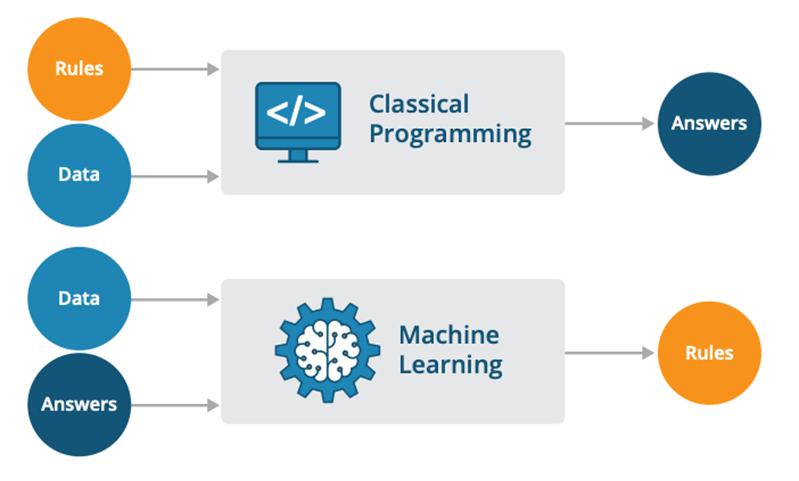
Machine Learning (ML) and traditional programming represent two fundamentally distinct approaches to solving tasks and making decisions.
- Traditional Programming: A human programmer explicitly defines the decision-making rules using if-then-else statements, logical rules, or algorithms.
- Machine Learning: The decision rules are inferred from data using learning algorithms.
- Traditional Programming: Inputs are processed according to predefined rules and logic, without the ability to adapt based on new data, unless these rules are updated explicitly.
- Machine Learning: Algorithms are designed to learn from and make predictions or decisions about new, unseen data.
- Traditional Programming: Suited for tasks with clearly defined rules and logic.
- Machine Learning: Well-adapted for tasks involving pattern recognition, outlier detection, and complex, unstructured data.
Here is the Python code:
def is_prime(num):
    if num < 2:
        return False
    for i in range(2, num):
        if num % i == 0:
            return False
    return True

print(is_prime(13))  # Output: True
print(is_prime(14)) # Output: FalseHere is the Python code:
from sklearn.model_selection import train_test_split
from sklearn.ensemble import RandomForestClassifier
from sklearn.datasets import load_iris
import numpy as np

# Load a well-known dataset, Iris
data = load_iris()
X, y = data.data, data.target
# Assuming 14 is the sepal length in cm for an Iris flower
new_observation = np.array([[14, 2, 5, 2.3]])
# Using Random Forest for classification
model = RandomForestClassifier()
model.fit(X, y)
print(model.predict(new_observation)) # Predicted classSupervised and Unsupervised Learning are two of the most prominent paradigms in machine learning, each with its unique methods and applications.
In Supervised Learning, the model learns from labeled data, discovering patterns that map input features to known target outputs.
-
Training: Data is labeled, meaning the model is provided with input-output pairs. It's akin to a teacher supervising the process.
-
Goal: To predict the target output for new, unseen data.
-
Example Algorithms:
- Decision Trees
- Random Forest
- Support Vector Machines
- Neural Networks
- Linear Regression
- Logistic Regression
- Naive Bayes
Here is the Python code:
from sklearn.model_selection import train_test_split
from sklearn.tree import DecisionTreeClassifier
from sklearn.metrics import accuracy_score

# Sample data - X represents features, y represents the target
X, y = data['X'], data['y']

# Split the data into training and testing sets
X_train, X_test, y_train, y_test = train_test_split(X, y, test_size=0.2)

# Initialize a Decision Tree classifier
classifier = DecisionTreeClassifier()

# Train the classifier using the training data
classifier.fit(X_train, y_train)

# Make predictions on the test data
predictions = classifier.predict(X_test)

# Evaluate the model
accuracy = accuracy_score(y_test, predictions)
print(f"Model accuracy: {accuracy}")In contrast to Supervised Learning, Unsupervised Learning operates with unlabelled data, where the model identifies hidden structures or patterns.
-
Training: No explicit supervision or labels are provided.
-
Goal: Broadly, to understand the underlying structure of the data. Common tasks include clustering, dimensionality reduction, and association rule learning.
-
Example Algorithms:
- K-Means Clustering
- Hierarchical Clustering
- DBSCAN
- Principal Component Analysis (PCA)
- Singular Value Decomposition (SVD)
- t-Distributed Stochastic Neighbor Embedding (t-SNE)
- Apriori
- Eclat
Here is the Python code:
from sklearn.cluster import KMeans

# Generate some sample data
X, _ = make_blobs(n_samples=300, centers=4, cluster_std=1.0, random_state=20)

# Initialize the KMeans object for k=4
kmeans = KMeans(n_clusters=4, random_state=42)

# Cluster the data
kmeans.fit(X)

# Visualize the clusters
visualize_clusters(X, kmeans.labels_)These paradigms serve as a bridge between the two primary modes of learning.
Semi-Supervised Learning makes use of a combination of labeled and unlabeled data. It's especially useful when obtaining labeled data is costly or time-consuming.
Reinforcement Learning often operates in an environment where direct feedback on actions is delayed or only partially given. Its goal, generally more nuanced, is to learn a policy that dictates actions in a specific environment to maximize a notion of cumulative reward.
Classification aims to categorize data into distinct classes or groups, while regression focuses on predicting continuous values.
- Examples: Email as spam or not spam, patient diagnosis.
- Output: Discrete, e.g., binary (1 or 0) or multi-class (1, 2, or 3).
- Model Evaluation: Metrics like accuracy, precision, recall, and F1-score.
- Examples: House price prediction, population growth analysis.
- Output: Continuous, e.g., a range of real numbers.
-
Model Evaluation: Metrics such as mean squared error (MSE) or coefficient of determination (
$R^2$ ).
In a classification problem, the output can be represented as:
whereas in regression, it can be a continuous value:
Here is the Python code:
# Import the necessary libraries
import numpy as np
from sklearn.linear_model import LogisticRegression, LinearRegression
from sklearn.model_selection import train_test_split
from sklearn.metrics import accuracy_score, mean_squared_error

# Generate sample data
X = np.random.rand(100, 1)
y_classification = np.random.randint(2, size=100)  # Binary classification target
y_regression = 2*X + 1 + 0.2*np.random.randn(100, 1)  # Regression target

# Split the data for both problems
X_train, X_test, y_class_train, y_class_test = train_test_split(X, y_classification, test_size=0.2, random_state=42)
_, _, y_reg_train, y_reg_test = train_test_split(X, y_regression, test_size=0.2, random_state=42)

# Instantiate the models
classifier = LogisticRegression()
regressor = LinearRegression()

# Fit the models
classifier.fit(X_train, y_class_train)
regressor.fit(X_train, y_reg_train)

# Predict the targets
y_class_pred = classifier.predict(X_test)
y_reg_pred = regressor.predict(X_test)

# Evaluate the models
class_acc = accuracy_score(y_class_test, y_class_pred)
reg_mse = mean_squared_error(y_reg_test, y_reg_pred)

print(f"Classification accuracy: {class_acc:.2f}")
print(f"Regression MSE: {reg_mse:.2f}")Overfitting and underfitting are two types of modeling errors that occur in machine learning.
- Description: The model performs well on the training data but poorly on unseen test data.
- Cause: Capturing noise or spurious correlations, using a model that is too complex.
- Indicators: High accuracy on training data, low accuracy on test data, and a highly complex model.
- Mitigation Strategies:
- Use a simpler model (e.g., switch from a complex neural network to a decision tree).
- Cross-Validation: Partition data into multiple subsets for more robust model assessment.
- Early Stopping: Halt model training when performance on a validation set decreases.
- Feature Reduction: Eliminate or combine features that may be noise.
- Regularization: Introduce a penalty for model complexity during training.
- Description: The model performs poorly on both training and test data.
- Cause: Using a model that is too simple or not capturing relevant patterns in the data.
- Indicators: Low accuracy on both training and test data and a model that is too simple.
- Mitigation Strategies:
- Use a more complex model that can capture the data's underlying patterns.
- Feature Engineering: Create new features derived from the existing ones to make the problem more approachable for the model.
- Increasing Model Complexity: For algorithms like decision trees, using a deeper tree or more branches.
- Reducing Regularization: for models where regularization was introduced, reducing the strength of the regularization parameter.
- Ensuring Sufficient Data: Sometimes, even the most complex models can appear to be underfit if there's not enough data to learn from. More data might help the model capture all the patterns better.
The goal is to find a middle ground where the model generalizes well to unseen data. This is often referred to as model parsimony or Occam's razor.
The Bias-Variance Tradeoff is a fundamental concept in machine learning that deals with the interplay between a model's predictive power and its generalizability.
-
Bias: Arises when a model is consistently inaccurate on training data. High-bias models typically oversimplify the underlying patterns (underfit).
-
Variance: Occurs when a model is highly sensitive to small fluctuations in the training data, leading to overfitting.
-
Irreducible Error: Represents the noise in the data that any model, no matter how complex, cannot capture.
- High-Bias Models: Are often too simple and overlook relevant patterns in the data.
- High-Variance Models: Are too sensitive to noise and might capture random fluctuations as real insights.
An ideal model strikes a balance between the two.
.png?alt=media&token=38240fda-2ca7-49b9-b726-70c4980bd33b)
- More Data: Generally reduces variance, but can also help a high-bias model better capture underlying patterns.
- Feature Selection/Engineering: Aims to reduce overfitting by focusing on the most relevant features.
- Simpler Models: Helps alleviate overfitting; reduces variance but might increase bias.
- Regularization: A technique that adds a penalty term for model complexity, which can help decrease overfitting.
- Ensemble Methods: Combine multiple models to reduce variance and, in some cases, improve bias.
- Cross-Validation: Helps estimate the performance of a model on an independent dataset, providing insights into both bias and variance.
Cross-Validation (CV) is a robust technique for assessing the performance of a machine learning model, especially when it involves hyperparameter tuning or comparing multiple models. It addresses issues such as overfitting and ensures a more reliable performance estimate on unseen data.
- Holdout Method: Data is simply split into training and test sets.
- K-Fold CV: Data is divided into K folds; each fold is used as a test set, and the rest are used for training.
- Stratified K-Fold CV: Like K-Fold, but preserves the class distribution in each fold, useful for balanced datasets.
- Leave-One-Out (LOO) CV: A special case of K-Fold where K equals the number of instances; each observation is used as a test set once.
- Time Series CV: Specifically designed for temporal data, where the training set always precedes the test set.
- Data Utilization: Every data point is used for both training and testing, providing a more comprehensive model evaluation.
- Performance Stability: Averaging results from multiple folds can help reduce variability.
- Hyperparameter Tuning: Helps in tuning model parameters more effectively, especially when combined with techniques like grid search.
Here is the Python code:
import numpy as np
from sklearn.model_selection import KFold

# Create sample data
X = np.array([[1, 2], [3, 4], [5, 6], [7, 8], [9, 10]])
y = np.array([1, 2, 3, 4, 5])

# Initialize K-Fold splitter
kf = KFold(n_splits=3)

# Demonstrate how data is split
fold_index = 1
for train_index, test_index in kf.split(X):
    print(f"Fold {fold_index} - Train set indices: {train_index}, Test set indices: {test_index}")
fold_index += 1Regularization in machine learning is a technique used to prevent overfitting, which occurs when a model is too closely fit to a limited set of data points and may perform poorly on new data. Regularization discourages overly complex models by adding a penalty term to the loss function used to train the model.
L1 regularization, also known as Lasso (Least Absolute Shrinkage and Selection Operator), adds the absolute values of the coefficients to the cost function. This encourages a sparse solution, effectively performing feature selection by potentially reducing some coefficients to zero.
L2 regularization, or Ridge regression, adds the squared values of the coefficients to the cost function. This generally helps to reduce the model complexity by constraining the coefficients, especially effective when many features have small or moderate effects.
Elastic Net is a hybrid of L1 and L2 regularization. It combines both penalties in the cost function and is useful for handling situations when there are correlations amongst the features or when you need to incorporate both attributes of L1 and L2 regularization.
Max Norm Regularization constrains the L2 norm of the weights for each neuron and is typically used in neural networks. It limits the size of the parameter weights, ensuring that they do not grow too large:
from keras.constraints import max_normThis can be particularly beneficial in preventing overfitting in deep learning models.
For Lasso and Ridge regression, you can use the respective classes from Scikit-learn’s linear_model module:
from sklearn.linear_model import Lasso, Ridge

# Example of Lasso Regression
lasso_reg = Lasso(alpha=0.1)
lasso_reg.fit(X_train, y_train)

# Example of Ridge Regression
ridge_reg = Ridge(alpha=1.0)
ridge_reg.fit(X_train, y_train)You can apply Elastic Net regularization using its specific class from Scikit-learn:
from sklearn.linear_model import ElasticNet

# Elastic Net combines L1 and L2 regularization
elastic_net = ElasticNet(alpha=1.0, l1_ratio=0.5)
elastic_net.fit(X_train, y_train)
Max Norm regularization can be specified for layers in a Keras model as follows:
from keras.layers import Dense
from keras.models import Sequential
from keras.constraints import max_norm

model = Sequential()
model.add(Dense(64, input_dim=8, kernel_constraint=max_norm(3)))
Here, the max_norm(3) constraint ensures that the max norm of the weights does not exceed 3.
Parametric and non-parametric models represent distinct approaches in statistical modeling, each with unique characteristics in terms of assumptions, computational complexity, and suitability for various types of data.
-
Parametric Models:
- Make explicit and often strong assumptions about data distribution.
- Are defined by a fixed number of parameters, regardless of sample size.
- Typically require less data for accurate estimation.
- Common examples include linear regression, logistic regression, and Gaussian Naive Bayes.
-
Non-parametric Models:
- Make minimal or no assumptions about data distribution.
- The number of parameters can grow with sample size, offering more flexibility.
- Generally require more data for accurate estimation.
- Examples encompass k-nearest neighbors, decision trees, and random forests.
-
Parametric Models
- Advantages:
- Inferential speed: Once trained, making predictions or conducting inference is often computationally fast.
- Parameter interpretability: The meaning of parameters can be directly linked to the model and the data.
- Efficiency with small, well-behaved datasets: Parametric models can yield highly accurate results with relatively small, clean datasets that adhere to the model's distributional assumptions.
- Disadvantages:
- Strong distributional assumptions: Data must closely match the specified distribution for the model to produce reliable results.
- Limited flexibility: These models might not adapt well to non-standard data distributions.
- Advantages:
-
Non-Parametric Models
- Advantages:
- Distribution-free: They do not impose strict distributional assumptions, making them more robust across a wider range of datasets.
- Flexibility: Can capture complex, nonlinear relationships in the data.
- Larger sample adaptability: Particularly suitable for big data or data from unknown distributions.
- Disadvantages:
- Computational overhead: Can be slower for making predictions, especially with large datasets.
- Interpretability: Often, the predictive results are harder to interpret in terms of the original features.
- Advantages:
Here is the Python code:
# Gaussian Naive Bayes (parametric)
from sklearn.naive_bayes import GaussianNB
model = GaussianNB()

# Decision Tree (non-parametric)
from sklearn.tree import DecisionTreeClassifier
model_dt = DecisionTreeClassifier()The curse of dimensionality describes the issues that arise when working with high-dimensional data, affecting the performance of machine learning models.
-
Sparse Data: As the number of dimensions increases, the data points become more spread out, and the density of data points decreases.
-
Increased Volume of Data: With each additional dimension, the volume of the sample space grows exponentially, necessitating a larger dataset to maintain coverage.
-
Overfitting: High-dimensional spaces make it easier for models to fit to noise rather than the underlying pattern in the data.
-
Computational Complexity: Many machine learning algorithms exhibit slower performance and require more resources as the number of dimensions increases.
Consider a hypercube (n-dimensional cube) inscribed in a hypersphere (n-dimensional sphere) with a large number of dimensions, say 100. If you were to place a "grid" or uniformly spaced points within the hypercube, you'd find that the majority of these points actually fall outside the hypersphere.
This disparity grows more pronounced as the number of dimensions increases, leading to a "density gulf" between the data contained within the hypercube and that within the hypersphere.
.png?alt=media&token=24d3cde6-89ae-4eb3-8d05-1d6358bb5ac9)
-
Feature Selection and Dimensionality Reduction: Prioritize quality over quantity of features. Techniques like PCA, t-SNE, and LDA can help reduce dimensions.
-
Simpler Models: Consider using algorithms with less sensitivity to high dimensions, even if it means sacrificing a bit of performance.
-
Sparse Models: For high-dimensional, sparse datasets, models that can handle sparsity, like LASSO or ElasticNet, might be beneficial.
-
Feature Engineering: Craft domain-specific features that can capture relevant information more efficiently.
-
Data Quality: Strive for a high-quality dataset, as more data doesn't necessarily counteract the curse of dimensionality.
-
Data Stratification and Sampling: When possible, stratify and sample data to ensure coverage across the high-dimensional space.
-
Computational Resources: Leverage cloud computing or powerful hardware to handle the increased computational demands.
Feature engineering is a vital component of the machine-learning pipeline. It entails creating meaningful and robust representations of the data upon which the model will be built.
-
Improved Model Performance: High-quality features can make even simple models more effective, while poor features can hamper the performance of the most advanced models.
-
Dimensionality Reduction: Carefully engineered features can distill relevant information from high-dimensional data, leading to more efficient and accurate models.
-
Model Interpretability: Certain feature engineering techniques, such as binning or one-hot encoding, make it easier to understand and interpret the model's decisions.
-
Computational Efficiency: Engineered features can often streamline computational processes, making predictions faster and cheaper.
-
Handling Missing Data
- Removing or imputing missing values.
- Creating a separate "missing" category.
-
Handling Categorical Data
- Converting categories into ordinal values.
- Using one-hot encoding to create binary "dummy" variables.
- Grouping rare categories into an "other" category.
-
Handling Temporal Data
- Extracting specific time-related features from timestamps, such as hour or month.
- Converting timestamps into different representations, like age or duration since a specific event.
-
Variable Transformation
- Using mathematical transformations such as logarithms.
- Normalizing or scaling data to a specific range.
-
Discretization
- Converting continuous variables into discrete bins, e.g., converting age to age groups.
-
Feature Extraction
- Reducing dimensionality through techniques like PCA or LDA.
-
Feature Creation
- Engineering domain-specific metrics.
- Generating polynomial or interaction features.
Data Preprocessing is a vital early-stage task in any machine learning project. It involves cleaning, transforming, and standardizing data to make it more suitable for predictive modeling.
-
Data Cleaning:
- Address missing values: Implement strategies like imputation or removal.
- Outlier detection and handling: Identify and deal with data points that deviate significantly from the rest.
-
Feature Selection and Engineering:
- Choose the most relevant features that contribute to the model's predictive accuracy.
- Create new features that might improve the model's performance.
-
Data Transformation:
- Normalize or standardize numerical data to ensure all features contribute equally.
- Convert categorical data into a format understandable by the model, often using techniques like one-hot encoding.
- Discretize continuous data when required.
-
Data Integration:
- Combine data from multiple sources, ensuring compatibility and consistency.
-
Data Reduction:
- Reduce the dimensionality of the feature space, often to eliminate noise or improve computational efficiency.
Here is the Python code:
# Drop rows with missing values
cleaned_data = raw_data.dropna()

# Fill missing values using the mean
mean_value = raw_data['column_name'].mean()
raw_data['column_name'].fillna(mean_value, inplace=True)Here is the Python code:
from sklearn.preprocessing import StandardScaler

scaler = StandardScaler()
X_train = scaler.fit_transform(X_train)
X_test = scaler.transform(X_test)Here is the Python code:
from sklearn.decomposition import PCA

pca = PCA(n_components=2)
X_pca = pca.fit_transform(X)Both Feature Scaling and Normalization are data preprocessing techniques that aim to make machine learning models more robust and accurate. While they share similarities in standardizing data, they serve slightly different purposes.
-
Feature Scaling adjusts the range of independent variables or features so that they are on a similar scale. Common methods include Min-Max Scaling and Standardization.
-
Normalization, in the machine learning context, typically refers to scaling the magnitude of a vector to make its Euclidean length 1. It's also known as Unit Vector transformation. In some contexts, it may be used more generally to refer to scaling quantities to be in a range (like Min-Max), but this is a less common usage in the ML community.
-
Min-Max Scaling: Transforms the data to a specific range (usually 0 to 1 or -1 to 1).
-
Standardization: Rescales the data to have a mean of 0 and a standard deviation of 1.
-
Unit Vector Transformation: Scales data to have a Euclidean length of 1.
-
Feature Scaling: Beneficial for algorithms that compute distances or use linear methods, such as K-Nearest Neighbors (KNN) or Support Vector Machines (SVM).
-
Normalization: More useful for algorithms that work with vector dot products, like the K-Means clustering algorithm and Neural Networks.
One-Hot Encoding is a technique frequently used to prepare categorical data for machine learning algorithms.
It is employed when:
- Categorical Data: The data on hand is categorical, and the algorithm or model being used does not support categorical input.
- Nominal Data Order: The categorical data is nominal, i.e., not ordinal, which means there is no inherent order or ranking.
-
Non-Scalar Representation: The model can only process numerical (scalar) data. The model may be represented as the set
$x = {x_1, x_2, \ldots, x_k}$ each$x_i$ corresponding to a category. A scalar transformation$f(x_i)$ or comparison$f(x_i) > f(x_j)$ is not defined for the categories directly. - Category Dimension: The categorical variable has many distinct categories. For instance, using one-hot encoding consistently reduces the computational and statistical burden in algorithms.
Here is the Python code:
import pandas as pd

# Sample data
data = pd.DataFrame({'color': ['red', 'green', 'blue', 'green', 'red']})

# One-hot encode
one_hot_encoded = pd.get_dummies(data, columns=['color'])
print(one_hot_encoded)| color_blue | color_green | color_red | |
|---|---|---|---|
| 0 | 0 | 0 | 1 |
| 1 | 0 | 1 | 0 |
| 2 | 1 | 0 | 0 |
| 3 | 0 | 1 | 0 |
| 4 | 0 | 0 | 1 |
| Color | Binary Red | Binary Green | Binary Blue |
|---|---|---|---|
| Red | 1 | 0 | 0 |
| Green | 0 | 1 | 0 |
| Blue | 0 | 0 | 1 |
Handling Missing Values is a crucial step in the data preprocessing pipeline for any machine learning or statistical analysis.
It involves identifying and dealing with data points that are not available, ensuring the robustness and reliability of the subsequent analysis or model.
-
Listwise Deletion: Eliminate entire rows with any missing value. This method is straightforward but can lead to significant information loss, especially if the dataset has a large number of missing values.
-
Pairwise Deletion: Ignore specific pairs of missing values across variables. While this method preserves more data than listwise deletion, it can introduce bias in the analysis.
-
Mean/ Median/ Mode: Replace missing values with the mean, median, or mode of the variable. This method is quick and easy to implement but can affect the distribution and introduce bias.
-
Forward or Backward Fill (Last Observation Carried Forward - LOCF / Last Observation Carried Backward - LOCB): Substitute missing values with the most recent (forward) or next (backward) non-missing value. These methods are useful for time-series data.
-
Linear Interpolation: Estimate missing values by fitting a linear model to the two closest non-missing data points. This method is particularly useful for ordered data, but it assumes a linear relationship.
-
k-Nearest Neighbors (KNN): Impute missing values based on the values of the k most similar instances or neighbors. This method can preserve the original data structure and is more robust than single imputation.
-
Expectation-Maximization (EM) Algorithm: Model the data with an initial estimate, then iteratively refine the imputations. It's effective for data with complex missing patterns.
- Use predictive models, typically regression or decision tree-based models, to estimate missing values. This approach can be more accurate than simpler methods but also more computationally intensive.
-
Understanding the Mechanism of Missing Data: Investigating why the data is missing can provide insights into the problem. For instance, is the data missing completely at random, at random, or not at random?
-
Combining Techniques: Employing multiple imputation methods or a combination of imputation and deletion strategies can help achieve better results.
-
Evaluating Impact on Model: Compare the performance of the model with and without the imputation method to understand its effect.
Feature Selection is a critical step in the machine learning pipeline. It aims to identify the most relevant features from a dataset, leading to improved model performance, reduced overfitting, and faster training times.
- Description: Filter methods rank features based on certain criteria, such as their correlation with the target variable or their variance.
- Advantages: They are computationally efficient and can be used in both regression and classification tasks.
- Limitations: They do not take feature dependencies into account.
- Description: Wrapper methods select features based on their performance with a specific machine learning algorithm. Common techniques include Recursive Feature Elimination (RFE) and Forward-Backward Selection.
- Advantages: They take feature dependencies into account and can improve model accuracy.
- Limitations: They can be computationally expensive and prone to overfitting.
- Description: Embedded methods integrate feature selection with the model building process. Techniques like LASSO (Least Absolute Shrinkage and Selection Operator) and decision tree feature importances are examples of this approach.
- Advantages: They are computationally efficient and provide feature rankings.
- Limitations: They may not be transferable to other models.
Here is the Python code:
import pandas as pd
from sklearn.feature_selection import VarianceThreshold

# Generate example data
data = {'feature1': [1, 2, 3, 4, 5],
        'feature2': [0, 0, 0, 0, 0],
        'feature3': [1, 0, 1, 0, 1],
        'target': [0, 1, 0, 1, 0]}
df = pd.DataFrame(data)

# Remove features with low variance
X = df.drop('target', axis=1)
y = df['target']
selector = VarianceThreshold(threshold=0.2)
X_selected = selector.fit_transform(X)

print(X_selected)Here is the Python code:
from sklearn.feature_selection import RFE
from sklearn.linear_model import LogisticRegression

# Create the RFE object and rank features
model = LogisticRegression(solver='lbfgs')
rfe = RFE(model, 3)
fit = rfe.fit(X, y)

print("Selected Features:")
print(fit.support_)
Explore all 100 answers here 👉 Devinterview.io - Data Scientist