
You can also find all 52 answers here 👉 Devinterview.io - Classification Algorithms
In the realm of Machine Learning, Classification empowers algorithms to categorize data into discrete classes or labels. It is utilized in an array of applications, from email filtering to medical diagnostics.
- Input: Utilizes a set of predefined features.
- Output: Assigns categories, or more frequently, predicts a discrete label.
- Training: Involves presenting the algorithm with a dataset, typically with known labels, to reinforce learning.
- Feedback Loop: Provides insight into the algorithm's accuracy and aids in refining its predictions over time.
The decision boundary is a hyperplane that demarcates separate classes in a feature space.
- Linear Boundaries: Employed in algorithms such as Power Iteration or Support Vector Machines.
- Non-Linear Boundaries: Algorithms like Decision Trees and Neural Networks can learn more complex boundary definitions.
A variety of metrics, including accuracy, precision, recall, and F1-score, are employed to gauge a classifier's efficiency.
- Medical Diagnostics: Separating tumors into benign or malignant categories.
- Email Filtering: Distinguishing between spam and genuine emails.
- Image Categorization: Assigning images to classes such as "cat" or "dog".
Binary Classification categorizes data into one of two classes, like "Yes" or "No", "True" or "False".
Multiclass Classification, on the other hand, deals with three or more classes.
- Binary Classification: Techniques can include Logistic Regression, Decision Trees, and Support Vector Machines.
- Multiclass Classification: Algorithms such as Decision Trees, k-Nearest Neighbors, and Linear Discriminant Analysis directly support multiclass classification. Techniques like One-Versus-Rest (OVR) and One-Versus-One (OVO) can also be used in combination with binary classifiers.
- Binary Classification: Typically employs loss functions like Logistic Loss (Log Loss) or Hinge Loss, which measure the accuracy of predicted probabilities against the true class label.
- Multiclass Classification: Uses appropriate loss functions, such as Cross-Entropy for comparing multiple classes with the predicted probabilities.
- Binary Classification: Common metrics include Accuracy, Precision, Recall, F1-Score, and Area Under the Receiver Operating Characteristic Curve (AUC-ROC).
- Multiclass Classification: Additionally evaluates using these metrics: Micro-Average, Macro-Average, and weighted averages for Precision, Recall, and F1-Score. Other metrics like Categorical Accuracy, Cohen's Kappa, or multiclass AUC may also be used.
-
Binary Classification: Predicting if an email is spam or not.
-
Multiclass Classification: Distinguishing multiple types of flowers based on their features or identifying different categories in images or textual data sets.
In supervised learning, a classification algorithm learns from a labeled dataset by using optimization techniques such as gradient descent to find the parameters that best separate classes.
-
Input Data: The algorithm ingests a labeled dataset, comprised of input features and corresponding class labels.
-
Data Preprocessing: This includes activities such as feature scaling, handling missing data, and splitting the dataset into training and test sets.
-
Initialization: Initial estimates of parameters are set, often randomly.
-
Prediction Generation: Based on initial parameter estimates, predictions are made for each data point, and an \textbf{objective function} is computed, capturing the algorithm's current level of "error."
-
Optimization: Using methods such as gradient descent, parameters are adjusted to minimize the objective function, and predictive accuracy is improved.
-
Convergence Check: The process is repeated until a stopping condition is met. This condition might be a maximum number of iterations or a specific level of accuracy or error rate.
-
Performance Metrics: Algorithms assess predictive accuracy using measures like precision, recall, and F1-score.
-
Generalization: The trained model's performance is evaluated on unseen data (the test set) to ensure it can make reliable predictions on new, incoming data.
-
Overfitting and Model Complexity: Techniques such as cross-validation are employed to guard against model overfitting and to determine the ideal level of model complexity.
Once trained, the model is ready for inference, where it makes predictions on new, unlabeled data for which the class label is unknown.
The outcome of the training process is an optimized set of parameters, known as the model. This model acts as a decision boundary, classifying new data points based on their input features.
Loss functions are pivotal in Classification algorithms as they quantify the disparity between predicted and actual values, enabling model optimization.
-
Mathematical Definition: Loss functions evaluate the discrepancy between target and prediction for a single instance through a mathematical formula, returning a scalar value. In classification, this entails assessing the class prediction.
-
Optimization Strategy: Classification algorithms aim to minimize the loss function, adjusting model parameters to enhance predictive accuracy.
-
Probabilistic Interpretation: In addition to offering a binary (True/False) decision, many classifiers, such as Logistic Regression and models in the Random Forest family, estimate the probability of the positive class. These probabilities are crucial for decision thresholds, especially in scenarios where asymmetric misclassification costs apply.
-
Weight Update Decision: Accurate prediction implies a lower loss and thus requires minimal or zero adjustment to model parameters. Introducing a loss function dictates how deviations contribute to parameter adjustments during training.
-
Stochastic Gradient Descent: For efficiency reasons, many classification algorithms, especially neural network-based ones, utilize algorithms like Stochastic Gradient Descent (SGD) to minimize the loss function over the entire dataset or data points in mini-batches.
-
Early Stopping & Cross-Validation: Beyond model development, loss functions empower decisions about model generalization, assisting actions like stopping training at an optimal epoch via early stopping or hyperparameter selection through cross-validation.
- Binary Classification: Applies the cross-entropy or log loss function.
Where
- Multi-Class Classification: Utilizes the categorical cross-entropy function, adjusted appropriately.
- Binary Classification: Employs the hinge loss function, aiming to separate class-specific decision boundaries.
-
Binary Classification: The Gini impurity or information gain measure is often utilized to make split decisions. While technically not a loss function, both these metrics serve as a heuristic to guide tree building. For Random Forests, individual trees have the freedom to work with different loss functions.
-
Multi-Class Classification: The Gini index or entropy can be extended to the multi-class case.
-
Probabilistic Output: Random Forests often use one-vs.-rest or averages to derive probabilities.
-
Binary Classification: Employs simple majority voting and doesn't require an explicit loss function. For probabilistic output, it adapts by returning the proportion of positive class neighbors.
-
Multi-Class Classification: It extends the majority voting concept.
Generative and Discriminative models, both used in the field of machine learning, have different ways of utilizing data and making predictions.
-
Generative: Learns the joint probability distribution of the input features and the target label, i.e.,
$P(X, Y)$ . -
Discriminative: Focuses on learning the conditional probability of the target label given the input features, i.e.,
$P(Y|X)$ .
-
Generative: Aims to model how data is generated to perform tasks such as recognition, classification, and unsupervised learning.
-
Discriminative: Primarily focuses on the decision boundary between classes for classification tasks.
-
Generative: Can handle missing data and naturally extend to new classes or data distributions.
-
Discriminative: The model sometimes struggles during application to data points or classes not seen during training.
-
Generative: Typically uses maximum likelihood estimation along with techniques like Expectation-Maximization in unsupervised learning tasks.
-
Discriminative: Often employs methods like logistic regression or support vector machines which are trained to directly optimize a discrimination function.
-
Generative: The Naive Bayes model, for instance, makes an independence assumption among features given the class, simplifying the modeling process.
-
Discriminative: Does not assume independence among the input features. Linear Discriminant Analysis (LDA) and Quadratic Discriminant Analysis (QDA) are examples of models that capture feature correlations to varying degrees.
-
Generative: Inherently suited for generating new, synthetic data (such as in GANs).
-
Discriminative: Typically lacks the ability to generate new data. Techniques like SMOTE are used to augment data, often in supervised learning settings.
Decision boundaries are fundamental to classification tasks. These are what algorithms use to discern between different classes.
When working in a two-dimensional feature space, decision boundaries are delineated as lines and curves that separate distinct classes.
Linear boundaries, such as lines or hyperplanes, are used when classes are well-discriminated and can be separated by a straight line in 2D or a plane in higher dimensions.
-
Polynomial: These create complex decision regions, but computationally may become cumbersome with higher degrees.
-
Piecewise Linear: Consist of multiple linear segments connected together, often forming shapes like triangles or trapezoids.
-
Radial Basis Functions (RBF): Typically represented as circles or ellipses, they are a classification method based on kernel theory.
-
Decision Trees: This leads to piecewise linear boundaries, but in 2D they might even look like steps or stairs.
Visualizing decision boundaries can greatly aid in understanding model behavior. This can be done using graphs, such as a contour plot, where different regions correspond to different classes.
Here is the Python code:
import numpy as np
import matplotlib.pyplot as plt
from sklearn import datasets
from sklearn.neighbors import KNeighborsClassifier
from mlxtend.plotting import plot_decision_regions

# Load iris dataset
iris = datasets.load_iris()
X = iris.data[:, :2]  # Use first two features for simplicity
y = iris.target

# Fit K-nearest neighbor classifier
knn = KNeighborsClassifier(n_neighbors=3)
knn.fit(X, y)

# Plot decision boundary
plot_decision_regions(X, y, clf=knn, legend=2)

# Show the plot
plt.xlabel(iris.feature_names[0])
plt.ylabel(iris.feature_names[1])
plt.title('K-NN Decision Boundary')
plt.show()When working with categorical features in a classification task, it's important to ensure they don't introduce bias or hinder model performance.
-
One-Hot Encoding: Transforms each category into a binary feature. While simple and intuitive, it can lead to the dummy variable trap.
-
Dummy Variable Coding: Setting one category as a reference, and using binary indicators for the others. This method is susceptible to imbalance between reference and non-reference levels.
-
Label Encoding: Assigns a unique integer to each category. This technique can mislead the algorithm that the categories have inherent order.
-
Count and Frequency Encoding: Replace categories with their occurrence counts or frequencies. This approach doesn't create additional features but can inflate the importance of frequent categories.
-
Target Encoding (Mean Encoding): Replace categories with the mean of the target variable for that category. This method is sensitive to overfitting and may not perform well on new data.
-
Weight of Evidence (WoE): It's used in credit scoring to encode categorical features, giving it a good informational value.
-
Binary-Based Encoder: Decompose the integer label for the category into binary code, which avoids the inherent order issue.
-
Embedding: Useful in deep learning and can capture complex, non-linear relationships.
-
Leave-One-Out Encoding: Replaces each category with the frequency of its occurrence except for the current observation.
-
Feature Hashing: Converts categories into a matrix of fixed size, which can be beneficial in case of limited computational resources.
-
Aggregating Levels: When categories have a hierarchical relationship, they can be grouped into broader levels.
-
Factorization: Reducing dimensionality through techniques like principal component analysis (PCA) or singular value decomposition (SVD). However, interpretability can be lost, especially with tree-based algorithms.
-
Clustering: Can group similar categories together, especially useful when there are many categories.
-
Decision Tree and Random Forest Importance: These methods offer insights into which features are most useful for classification.
Expert Knowledge, as well as domain understanding, is crucial to choosing the most effective combination of techniques for your specific problem.
For example, in credit scoring, it's common to use a combination of techniques, including Weight of Evidence, target encoding, and frequency-based encoding.
Similarly, in healthcare, methods like expert reasoning, feature selection, and imputation strategies guided by clinical knowledge can enhance model performance. Balancing rigor with interpretability is key in the context of healthcare decision-making.
-
Scikit-Learn: Utilize techniques such as one-hot-encoding, label-encoding, and target encoding. It also supports pipelines for systematic data preprocessing.
-
XGBoost: Default support for categorical features, which can be further optimized using techniques like target encoding.
-
Deep Learning Frameworks: They incorporate embedding layers, specifically designed for handling categorical features in neural networks.
-
Categorical Feature Selection: Machine learning libraries like XGBoost and LightGBM offer explicit support for categorical feature selection.
-
LIME and SHAP: These techniques provide post-hoc interpretability and can be used to deconstruct the complex relationship between encoded categorical features and target variables.
Prioritize data privacy and ethics while handling sensitive categorical features. Techniques like symmetric hashing help anonymize data, providing an added layer of protection.
Remember, the key to maximizing the predictive potential of categorical features lies in a widely-informed, evidence-based approach, customized to the unique context of the problem at hand.
The Curse of Dimensionality refers to challenges that arise when working with data in high-dimensional spaces. In the context of classification, it can make distance-based methods less reliable and hinder the performance of machine learning models.
As the number of dimensions
In high dimensions, the concept of distance becomes ambiguous. This stems from the fact that the relative difference between the lengths of different
The sparsity in high-dimensional data can distort the true distribution, leading to increased overfitting and decreased generalization accuracy. Moreover, the distortion can affect data points' relative positions, potentially causing neighboring points to become disjoint.
Several techniques aim to mitigate the challenges associated with high-dimensional spaces:
-
Feature Selection and Dimensionality Reduction: Identifying and using the most informative features can improve model performance. Techniques like Principal Component Analysis
$(PCA)$ or methods that consider feature importances, such as gain in XGBoost, can help reduce redundant or noisy information. -
Regularization: Incorporating regularization into machine learning models, such as
$L1$ or$L2$ regularization, can prevent overfitting by constraining the coefficients associated with less informative features. -
Distance Metric Customization: For distance-based classifiers, like k-Nearest Neighbors
$(k-NN)$ , customizing the distance metric to match the specific data distribution can enhance model accuracy. -
Model and Algorithm Selection: Some models and algorithms are intrinsically more robust in high-dimensional spaces. For instance, tree-based methods often handle a large number of features effectively.
-
Curse-Aware Validation Techniques: Employing advanced cross-validation methods, like k-fold cross-validation, ensures that model performance estimates are more consistent with real-world application. This is especially useful when dealing with high-dimensional data.
-
Consider Feature Interactions: In high-dimensional spaces, feature interactions can be complex. Accounting for these interactions, especially in non-linear models, can be beneficial.
-
Leverage External Information: Supplementing the dataset with external information to guide the learning process can help improve model performance, even in a high-dimensional context.
Logistic Regression may be somewhat of a misnomer, as it's actually a classification algorithm. It determines the likelihood of an instance belonging to a certain category.
Logistic Regression models the probability of an event occurring (binary classification, 0 or 1) or a particular class being present (multi-class classification), based on one or more features.
For a two-class scenario, a probability
where
The predicted class
- If
$p \geq 0.5$ , it's predicted as Class 1. - If
$p < 0.5$ , it's predicted as Class 0.
The separating line or rule that distinguishes between the classes in the feature space is known as the decision boundary.
One of the key distinctions of Logistic Regression is its ability to output probabilistic measures. This feature, combined with the choice of a cutoff value (typically 0.5), allows for a more nuanced understanding of model confidence and performance.
-
Linearity: The log odds of the target variable being equivalent to a linear combination of the predictor variables.
-
Independence: The observations should be independent of each other.
-
Absence of Multicollinearity: The features shouldn't be highly correlated with each other.
-
Large Dataset: It's ideal to have a large dataset for logistic regression.
-
Binary Dependent Variable: The dependent variable should be binary.
Logistic Regression is optimized using the Sigmoid Cross Entropy loss function. The aim is to minimize the difference between predicted probabilities and actual classes during training.
The Sigmoid Cross Entropy loss function is given by:
where:
-
$y$ represents the actual class label (0 or 1). -
$p$ represents the predicted probability from the Sigmoid function.
Here is the Python code:
import numpy as np

def sigmoid(z):
    return 1 / (1 + np.exp(-z))

# Example
z = np.array([1, 2, 3])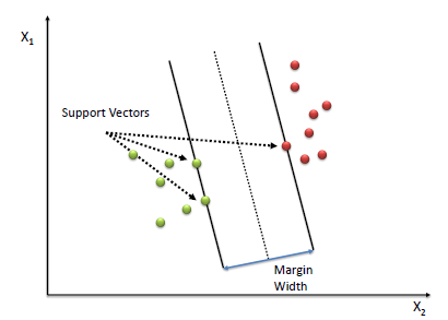
print(sigmoid(z))Support Vector Machines, or SVM, is a powerful supervised learning algorithm used for classification tasks.
-
SVM aims to find the best hyperplane that separates data points into different classes.
-
The "best" hyperplane is the one that maximizes the margin between the two classes. The margin is the distance between the hyperplane and the nearest data point from each class, often referred to as support vectors.
-
If the data is not linearly separable, SVM can still handle it through the use of kernels, which map the data into higher dimensions where separation is feasible.

The hyperplane equation can be expressed as:
Where
The margin between the two classes is given by:
The goal during optimization is to maximize this margin.
- Features Normalization: SVMs benefit from feature scaling.
- Handling Imbalanced Data: Techniques like cost-sensitive learning or resampling methods can be used.
- Model Evaluation: Common metrics like accuracy, precision, recall, and F1-score are used with SVM.
Here is the Python code:
from sklearn.svm import SVC
from sklearn.model_selection import train_test_split
from sklearn.metrics import accuracy_score
from sklearn.datasets import load_iris

# Load Iris dataset
iris = load_iris()
X, y = iris.data, iris.target

# Split data
X_train, X_test, y_train, y_test = train_test_split(X, y, test_size=0.3, random_state=42)

# Create an SVM model
model = SVC(kernel='linear')

# Train the model
model.fit(X_train, y_train)

# Make predictions
y_pred = model.predict(X_test)

# Calculate accuracy
accuracy = accuracy_score(y_test, y_pred)
print("Accuracy:", accuracy)Naive Bayes (NB) is a family of simple yet powerful probabilistic classifiers based on Bayes' theorem. It's often used for text classification in scenarios such as spam detection, sentiment analysis, and document categorization.
-
Bayes' Theorem: The fundamental statistical principle on which NB is built. It describes how to update the probability of a hypothesis given evidence.
-
Independence Assumption: The "naive" component of NB. It assumes that features are conditionally independent given the class label.
-
Prediction Method: NB selects the class with the highest a posteriori probability using Bayes' theorem.
-
Likelihood Computation: In NB, the likelihood is computed as the probability of observing each feature given the class.
-
Model Flexibility: While not as sophisticated as some other classifiers, NB is known for its efficiency and ability to handle large feature spaces.
For a feature set
Upon sampling,
Using the Independence Assumption, the probability simplifies to:
Here,
-
$Count(X_i, C)$ is the number of times feature$x_i$ occurs in instances of class$C$ . -
$|X|$ is the total number of unique features. -
$Count(C)$ is the total count of class$C$ .
Here is the Python code:
from sklearn.datasets import fetch_20newsgroups
from sklearn.feature_extraction.text import TfidfVectorizer
from sklearn.naive_bayes import MultinomialNB
from sklearn.model_selection import train_test_split
from sklearn.metrics import accuracy_score, classification_report

# Load text data
categories = ['alt.atheism', 'soc.religion.christian', 'comp.graphics', 'sci.med']
newsgroups_train = fetch_20newsgroups(subset='train', categories=categories)
newsgroups_test = fetch_20newsgroups(subset='test', categories=categories)
X_train = newsgroups_train.data
X_test = newsgroups_test.data
y_train = newsgroups_train.target
y_test = newsgroups_test.target

# Feature extraction and train-test split
tfidf = TfidfVectorizer()
X_train_tfidf = tfidf.fit_transform(X_train)
X_test_tfidf = tfidf.transform(X_test)

# Initialize and train NB classifier
nb_classifier = MultinomialNB()
nb_classifier.fit(X_train_tfidf, y_train)

# Predict and evaluate
y_pred = nb_classifier.predict(X_test_tfidf)
print('Accuracy:', accuracy_score(y_test, y_pred))
print(classification_report(y_test, y_pred, target_names=newsgroups_test.target_names))Decision Trees are non-linear models that partition the feature space into segments, making them advantageous for both classification and regression tasks.
A tree consists of:
- Root Node: No incoming edges. Represents the entire dataset.
- Internal Nodes: Subsets of the data based on feature conditions.
- Leaf Nodes: Terminal nodes that represent unique classes or regression outputs.
The decision of how to split the data at each node is based on selecting the feature and the threshold that yields the best binary subdivision. This optimization is performed using techniques like the Gini index or information gain.
-
Gini Index measures misclassification and is summed over all classes.
- Gini for a class
$k$ in a node$m$ :
- Gini for a class
-
Information Gain quantifies the reduction in entropy. It aims to create subsets that are more pure in terms of the target variable's class distribution.
- Entropy of node
$m$ :
- Entropy of node
- Information Gain for a feature
$A$ and node$m$ :
...where
- Root Node Selection: Identifies the initial best split.
- Splitting Criteria: Uses Gini impurity, Information Gain, or another criterion to determine the feature and threshold for best division.
- Termination: Establishes a stopping point, such as reaching a node purity threshold or a maximum tree depth.
- Recursive Splitting: Segments the data into partitions and repeats the process on each subset.
Here is the Python code:
# Import the necessary libraries
from sklearn import datasets
from sklearn.model_selection import train_test_split
from sklearn.tree import DecisionTreeClassifier
from sklearn.metrics import accuracy_score

# Load the dataset
iris = datasets.load_iris()
X, y = iris.data, iris.target

# Split the dataset
X_train, X_test, y_train, y_test = train_test_split(X, y, test_size=0.2, random_state=42)

# Initialize the model
dt_classifier = DecisionTreeClassifier(criterion='gini', max_depth=3, random_state=42)

# Fit the model to the training data
dt_classifier.fit(X_train, y_train)

# Make predictions on the test data
y_pred = dt_classifier.predict(X_test)

# Evaluate the model
accuracy = accuracy_score(y_test, y_pred)

print(f"Decision Tree Classifier accuracy: {accuracy}")Random Forest (RF) is an ensemble learning method comprised of multiple decision trees. It's frequently preferred over standalone decision trees due to its performance advantages, generalizability, and resilience to overfitting.
- Function: Divides the dataset into increasingly pure subsets based on feature criteria.
- Limitation: Prone to overfitting, especially in high-dimensional feature spaces.
- Function: Utilizes bootstrapping to build multiple trees from different, random subsets of the data.
- Function: Each node in a decision tree uses only a random subset of features. This practice, also known as "feature bagging," helps trees become more diverse from one another, reducing correlation.
- Collective Wisdom: By aggregating predictions from multiple trees, RF is more robust against outliers and noisy data than single decision trees.
- Gini Importance Metric: RF assesses the benefit of features during training, enabling better feature selection and pruning of less effective variables.
- Diversification: Emphasis on feature and data randomness promotes diverse tree structures, naturally lessening the risk of overfitting.
- Bootstrapped Sampling: Constituent trees are built from randomly resampled subsets of the data.
- Random Subset of Features: At each node, a feature subset is randomly chosen for the splitting criterion.
- Voting Mechanism: Binary or majority voting determines class predictions.
Here is the Python code:
from sklearn.ensemble import RandomForestClassifier
from sklearn.model_selection import train_test_split
from sklearn.datasets import load_iris
from sklearn.metrics import accuracy_score

# Load dataset
iris = load_iris()
X, y = iris.data, iris.target

# Split data
X_train, X_test, y_train, y_test = train_test_split(X, y, test_size=0.2)

# Instantiate RF classifier
rf_clf = RandomForestClassifier(n_estimators=100, random_state=42)

# Train model
rf_clf.fit(X_train, y_train)

# Make predictions
y_pred = rf_clf.predict(X_test)

# Calculate accuracy
accuracy = accuracy_score(y_test, y_pred)
print(f"Random Forest Classifier accuracy: {accuracy * 100:.2f}%")Gradient Boosting Machines (GBM) are a class of iterative ensemble learners that build models such as Decision Trees in a stage-wise manner. Unlike bagging methods that build multiple trees independently, each tree in GBM is trained to correct the errors of the previous one.
- Sequential Learning: Trees are added one at a time in an adaptive manner.
- Error-Focused Training: Each subsequent tree aims to minimize residual errors from the ensemble.
- Regularization Techniques: GBM often employs strategies to prevent overfitting, such as tree depth control and shrinkage (learning rate).
- Generate Initial Model: A simple, default prediction is made, often the mean of the target variable. Subsequent trees will correct the errors of this model.
- Compute Residuals: The difference between predictions and actual target values gives the residuals that need to be minimized by successive trees.
- Train Tree on Residuals: Using the residuals from the previous step as the new target, a new decision tree is created.
- Update Model with New Tree: The new tree's predictions are incorporated into the ensemble, along with a fraction of its learning rate.
- Repeat Steps 2-4: The process is iterative; additional trees refine the predictions further.
- High Accuracy: GBM is robust and typically yields high predictive abilities.
- Adaptive to Different Data Types: It handles both numerical and categorical variables.
- Effective Feature Selection: Attributes may be ranked based on their contribution to the decision trees.
- Computationally Demanding: GBM training can be time-consuming and resource-intensive.
- Prone to Overfitting: Without proper tuning, it can memorize the training data.
Here is the Python code:
from sklearn.ensemble import GradientBoostingClassifier
from sklearn.model_selection import train_test_split
from sklearn.metrics import accuracy_score

# Sample Data
X, y = load_dataset()

# Train-Test Split
X_train, X_test, y_train, y_test = train_test_split(X, y, test_size=0.2, random_state=42)

# Initialize GBM
model = GradientBoostingClassifier()

# Train Model
model.fit(X_train, y_train)

# Make Predictions
y_pred = model.predict(X_test)

# Evaluate Accuracy
accuracy = accuracy_score(y_test, y_pred)k-Nearest Neighbours (k-NN) is a simple yet powerful classification algorithm.
-
Determine K Value: Choose the number of nearest neighbors, denoted as
$k$ . -
Calculate Distances: Measure the distance between the target point and all other points in the dataset.
-
Pick the Nearest K Points: Select the K points in the training data that are closest to the target point based on distance metrics like Euclidean distance for continuous features.
$$d(x, y) = \sqrt{(x_1 - y_1)^2 + (x_2 - y_2)^2 + \ldots + (x_n - y_n)^2}$$ -
Majority Voting: From the K selected points, assign the class that most frequently occurs.
-
Classify the Unknown Point: Allocate the most common class as the predicted class label for the new data point.
- Adaptability: It's a non-parametric, instance-based method, meaning the model adapts to new data in real-time.
- Robust to Noisy Data: Its performance is generally unaffected by noisy instances or outliers.
- Interpretability: The method is straightforward to understand, as predictions are based on the nearest data points.
- Computational Overhead: Can be computationally expensive, especially with large datasets, as it needs to compute the distances to all points.
- Memory Intensive: Stores the complete dataset, requiring more memory as the dataset size grows.
-
Sensitive to K-Value: The algorithm's performance can be sensitive to the choice of
$k$ .
On a 2D plane, the algorithm divides the feature space into regions based on the different classes.

Each point's class is predicted based on the majority class of its
Here is the Python code:
from sklearn.datasets import load_iris
from sklearn.model_selection import train_test_split
from sklearn.preprocessing import StandardScaler
from sklearn.neighbors import KNeighborsClassifier
from sklearn.metrics import accuracy_score

# Load the dataset
iris = load_iris()
X, y = iris.data, iris.target

# Preprocess the data
scaler = StandardScaler()
X = scaler.fit_transform(X)

# Split the dataset
X_train, X_test, y_train, y_test = train_test_split(X, y, test_size=0.3, random_state=42)

# Initialize the k-NN model
k = 3  # Example k-value
knn = KNeighborsClassifier(n_neighbors=k)

# Fit the model to the training data
knn.fit(X_train, y_train)

# Make predictions on the test data
y_pred = knn.predict(X_test)

# Evaluate the model's accuracy
accuracy = accuracy_score(y_test, y_pred)
print(f"Accuracy: {accuracy*100:.2f}%")
Explore all 52 answers here 👉 Devinterview.io - Classification Algorithms