Main importations
import bloch as b  # a Class which is implemented in it`s own module
import numpy as np
from matplotlib.animation import FuncAnimation
import mpl_toolkits.mplot3d.axes3d as p3
from matplotlib import animation
import matplotlib.pyplot as plt
%matplotlib notebook
%matplotlib notebook
instantiation of the main class responsible for the calculations needed and printing the accompanied doc string
the file can be tracked here Bloch
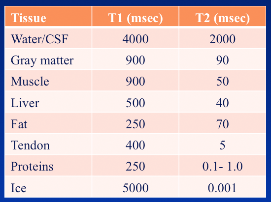
m = b.magentization(900*10**-3, 50*10**-3, 1.5)
print(b.magentization.__doc__)
Responsible for calculating the magnetization vector.
Implements the following:
* calculate the magnetization vector after application of Mo [0 0 Mo]
* Returns the vector into its relaxation state
the values we tried are from this link
m.rotate(1)
print(m.rotate.__doc__)
Rotates the magnetization vector by application of an RF pulse for a given time t
================== =================================================
**Parameters**
t Time in seconds
================== =================================================
The following chunk of code is responsible for making an animation of the bulk magnetization`s trajectory
- using matplotlib funcAnimation and quiver for 3d plotting
- the plot is initialized with the first values returned from the rotations of the vector
- an update function is given for FuncAnimation which updates the plot`s data with the next value to show in the next frame
fig = plt.figure()
ax = fig.gca(projection='3d')

# Origin
x, y, z = (0, 0, 0)

# Directions of the vector
u = m.vector[0, 0]  # x Component
v = m.vector[0, 1]  # y Component
w = m.vector[0, 2]   # z Component

quiver = ax.quiver(x, y, z, u, v, w, arrow_length_ratio=0.1, color="red")
ax.plot(m.vector[:0, 0], m.vector[:0, 1], m.vector[:0, 2], color='r', label="Trajectory")

def update(t):
    global quiver
    u = m.vector[t, 0]
    v = m.vector[t, 1]
    w = m.vector[t, 2]
    quiver.remove()
    quiver= ax.quiver(x, y, z, u, v, w, arrow_length_ratio=0.1)
    ax.plot(m.vector[:t, 0], m.vector[:t, 1], m.vector[:t, 2], color='r', label="Trajectory")

ax.set_xlim3d([-0.3, 0.3])
ax.set_xlabel('X')

ax.set_ylim3d([-0.3, 0.3])
ax.set_ylabel('Y')

ax.set_zlim3d([-1.5, 1.5])
ax.set_zlabel('Z')

ax.view_init(elev= 0.9, azim=-45)
ani = FuncAnimation(fig, update, frames=np.arange(0, 100), interval=200, blit= True)
ax.legend()
ani.save("magnetization.gif")
plt.show()the Animation

importing a class made for the image's loading and performing Fourier transform
import image # a class for image`s processes imageSlice = image.image()
print(image.image().__doc__) Responsible for all interactions with images.
Implements the following:
* Loading the image data to the class
* Apply Fourier Transformation to the image
* Extract the following components from the transformations :
- Real Component
- Imaginary Component
- Phase
- Magnitude
imageSlice.loadImage("78146.png", greyScale=False)
print(imageSlice.loadImage.__doc__)
the image loaded shape is (230, 230, 3)
Implements the following:
* Loading the image from specified path
* Normalize the image values
================== =============================================================================
**Parameters**
Path a string specifying the absolute path to image, if provided loads this image
to the class`s data
data numpy array if provided loads this data directly
fourier numpy array if provided loads the transformed data
imageShape a tuple of ints identifying the image shape if any method is used except using
path
greyScale if True the image is transformed to greyscale via OpenCV`s convert image tool
================== =============================================================================
import matplotlib.cm as cmfig2 = plt.figure()
plt.title("Loaded Image/ Ankle")
plt.axis("off")
plt.imshow(imageSlice.imageData, cmap=cm.gray)
imageSlice.fourierTransform()
fig3 = plt.figure()
plt.title("Real K-Space Component")
plt.ylabel("Ky")
plt.xlabel("Kx")
plt.imshow(imageSlice.realComponent(logScale=True))
fig4 = plt.figure()
plt.title("Imaginary K-Space Component")
plt.ylabel("Ky")
plt.xlabel("Kx")
plt.imshow(imageSlice.phase(), cmap=cm.gray)
print("Function`s description")
print("imageSlice.fourierTransform: ")
print(imageSlice.fourierTransform.__doc__)
print("imageSlice.magnitude:")
print(imageSlice.magnitude.__doc__)
print("imageSlice.phase: ")
print(imageSlice.phase.__doc__)
Function`s description
imageSlice.fourierTransform:
Applies Fourier Transform on the data of the image and save it in the specified attribute
================== ===========================================================================
**Parameters**
shifted If True will also apply the shifted Fourier Transform
================== ===========================================================================
imageSlice.magnitude:
Extracts the image`s Magnitude Spectrum from the image`s Fourier data
================== ===========================================================================
**Parameters**
LodScale If True returns 20 * np.log(ImageFourier)
================== ===========================================================================
**Returns**
array a numpy array of the extracted data
================== ===========================================================================
imageSlice.phase:
Extracts the image`s Phase Spectrum from the image`s Fourier data
================== ===========================================================================
**Parameters**
shifted If true applies a phase shift on the returned data
================== ===========================================================================
**Returns**
array a numpy array of the extracted data
================== ===========================================================================
field = 3.0  # Tesla
delta = 0.5
Bz = np.random.uniform(field-delta, field+delta, size=10)fig5 = plt.figure()
plt.title("Magnetic Field`s Randomality")
plt.xlabel("Measured Point")
plt.ylabel("The Measured Field")
plt.hlines(3,0, 10, label="The Field Value")
plt.scatter(range(0, 10), Bz, label="Different Measured points")
plt.legend()
G = 42.6  # for water molecules
omega = G* Bz
fig6 = plt.figure()
plt.title("Angular Frequencies")
plt.xlabel("Measured Point")
plt.ylabel("Frequency(MHZ)")
plt.hlines(3*G,0, 10, label="The Field Value")
plt.scatter(range(0, 10), omega, label="Different Measured Frequencies")
plt.legend()
plt.show()m2 = b.magentization(T1, T2, Bz[:5])m2.rotate(1)fig = plt.figure()
ax = fig.gca(projection='3d')
# Origin
x = np.zeros(5)
y = np.zeros(5)
z = np.zeros(5)
colors = ['r', 'b', 'y', 'g', 'c']
# Initizalizing plot
# Directions of the vector m2
u = m2.vector[0, 0] # x Component
v = m2.vector[0, 1] # y Component
w = m2.vector[0, 2] # z Component
quiver = ax.quiver(x, y, z, u, v, w, arrow_length_ratio=0.1, color="red")
for point in range(5):
ax.plot(m2.vector[:0, 0, point], m2.vector[:0, 1, point], m2.vector[:0, 2, point], color=colors[point], label="Trajectory %s"%(point+1))
def update(t):
global quiver
u = m.vector[t, 0]
v = m.vector[t, 1]
w = m.vector[t, 2]
quiver.remove()
quiver= ax.quiver(x, y, z, u, v, w, arrow_length_ratio=0.1)
for point in range(5):
ax.plot(m2.vector[:t, 0, point], m2.vector[:t, 1, point], m2.vector[:t, 2, point],
color=colors[point], label="Trajectory %s"%(point+1))
ax.set_xlim3d([-0.3, 0.3])
ax.set_xlabel('X')
ax.set_ylim3d([-0.3, 0.3])
ax.set_ylabel('Y')
ax.set_zlim3d([-1.5, 1.5])
ax.set_zlabel('Z')
ax.view_init(elev= 28, azim=-45)
ani = FuncAnimation(fig, update, frames=np.arange(0, 100), interval=200, blit= True)
ax.legend()
ani.save("magnetization2.gif")
plt.show()