
Stalefish is a tool for the analysis of 2D brain slice images, allowing the neurobiologist to reconstruct three dimensional gene expression surfaces from ISH slices. The 3D surfaces can then be digitally unwrapped to make 2D expression maps. A paper giving a detailed description of the process is available from PNAS. There is also an open-neuroscience.com YouTube video about Stalefish and the history of its development as well as the associated video slides.
You start with a standard set of brain slice images. These are configured as a project and opened with stalefish. Sample collection curves are added to the images as a manual process using keyboard & mouse (Fig 1A). When the curves are arranged in a stack, a three dimensional surface can be created, as shown in Fig. 1B.
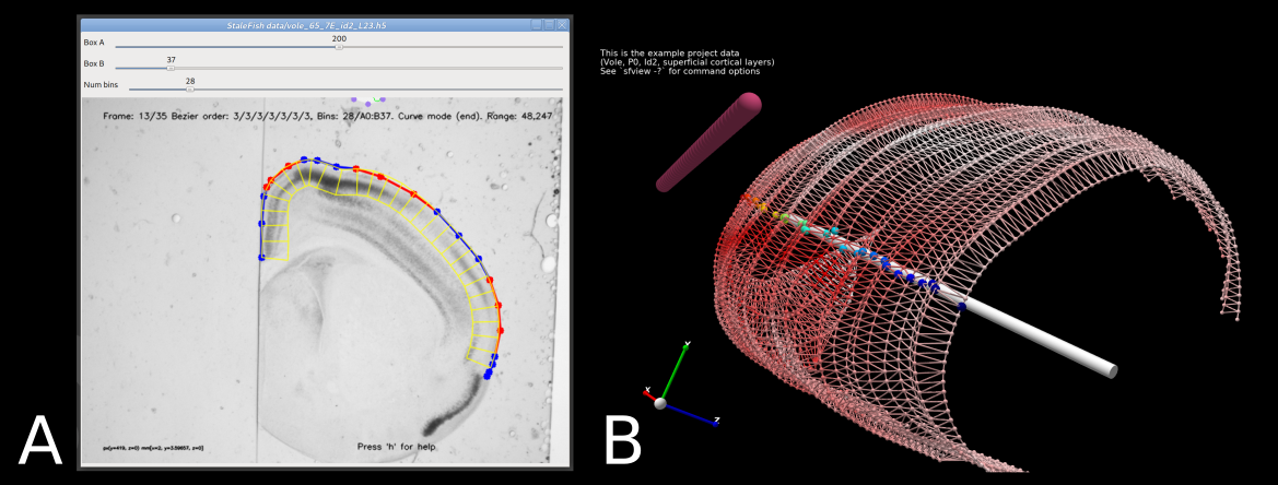 Figure 1: A User provided points (red and blue) define a curve from which yellow sampling bins are derived. The mean luminance in the sample bins gives data points for, in this case, the level of expression of a gene called 'Id2' at evenly spaced locations along the curve. B By arranging adjacent curves, the gene expression data forms a 3D surface, shown here as a mesh of spheres at the data points (rendered with sfview). The line of pink spheres give the position of alignment marks used to help align adjacent brain slices.
The surface can now be digitally unwrapped and resampled to produce a two dimensional image of the gene expression. Fig. 2 shows the sequence in which this is carried out. Once the map has been unwrapped, the patterns of gene expression can be analysed with standard image analysis tools.
 Figure 2: Three dimensions to two dimensions. A A filled render of the mesh in Fig. 1B. B Unwrapping the surface C Unwrapped surface shown as 2D map D The 2D map resampled so that it can be manipulated as a digital image.
The quickest way to try Stalefish is to install a pre-built image. (For build instructions see Building Stalefish.)
To install on Mac OS, download the Stalefish.dmg file from https://github.com/ABRG-Models/Stalefish/releases/
We've packaged Stalefish for Linux using 'snap'. This is a way to make apps available to many different distributions of Linux. If you have snapd installed on your system (it comes pre-installed in Ubuntu), you can install Stalefish with
sudo snap install stalefish
For help installing, see https://snapcraft.io/stalefish
Stalefish has a very simple user interface. In order to keep the code as small as possible, we haven't linked to any of the 'desktop widget' libraries such as Qt, Cocoa or GTK. That means we don't have access to common interfaces such as a file-chooser widget or application menus. We control the setup of the program using a text based configuration file written in a very friendly format called JSON. This means that the path to the JSON file has to be provided on the command line when launching Stalefish like this:
./build/src/stalefish ./data/testimg.json
The JSON file contains a list of the images to fit curves to, and some other parameters. If you already have a Stalefish project file (these are HDF5 files), then the program call is:
./build/src/stalefish ./data/testimg.h5
If you launch Stalefish without the path, or from its program icon, you'll see a help screen and the option to open an example project by pressing the 'e' key.
Launch Stalefish with no path and press the 'e' key. You should now see a brain slice image in a window, with three sliders at the top of the window (Fig. 1A). The first task is to add or modify the points that will define the sampling curves that you'll build your 3D expression maps from. Stalefish has a concept of 'input modes' and the default mode is 'Curve mode'.
In Curve mode, a mouse click will create green points to which a curve should be fit. Create 3, 4 or 5 points then press 'space'. The points should turn blue (or red). Pressing space 'locks in' a section of the curve. Repeat to create a complete, smooth curve along an anatomical feature of interest. When you are satisfied, press 'f' to fit the curve. A green fit line and yellow sample bins should appear. Sliders give control over the size and shape of the sample bins. Now move on to the next slice in the set with 'n' and draw a curve on the same anatomical feature (assuming it spans several slices).
You can press 'h' to see help text detailing the key-press commands that are available. A more detailed description of the Stalefish application is available here: https://github.com/ABRG-Models/Stalefish/blob/master/docs/Supplement.pdf.
Stalefish projects are created with a hand-written .json file which lists the images in your brain slice set, along with some additional information, such as the position of each slice in the stack, the slice thickness and so on.
Example json files can be found in the data/ directory - see testimg.json and vole_65_7E_id2_L23.json.
There is also a program called sfmakejson which will generate a .json config file from a set of brain slice images. Here is an example call in which the slice thickness and the slice-to-slice distance are set to 0.1 mm and the scale of the slice images is 200 pixels per mm:
sfmakejson -d 0.1 -t 0.1 -p 200 ./brainslices/*.png > newproject.jsonNote that the standard digital output of sfmakejson is redirected into a new file called newproject.json.
The utility sfgetjson extracts the .json config file from a Stalefish .h5 project file. Note that these utilities are called stalefish.sfmakejson and stalefish.sfgetjson if you installed Stalefish using Snap (https://snapcraft.io/stalefish).
- pixels_per_mm Set to the number of pixels per mm in the original image files.
- thickness The thickness of a brain slice (in mm), assuming they'll all be the same.
- bg_blur_screen_proportion: Float. Typically 1/6 (0.1667). The sigma for the Gaussian used to blur the image to get the overall background luminance is the framewidth in pixels multiplied by this number.
- bg_blur_subtraction_offset: Float. Range 0.0 to 255.0. Typically 180. A subtraction offset used when subtracting blurred background signal from image
- colourmodel: Enumerated. Options are monochrome (default) or Allen
- colour_rot Array related to Allen colour images
- colour_trans Array related to Allen colour images
- ellip_axes Array (of 2 numbers) related to Allen colour images
- luminosity_cutoff: Float. No longer used in monochrome mode.
- luminosity_factor: Float. No longer used in monochrome mode.
- save_per_pixel_data: Boolean. If true, save coordinates and signal value for every pixel in every sample box. Inflates .h5 file somewhat
- save_auto_align_data: Boolean. If true, save the slice auto-alignment location data
- save_landmark_align_data: Boolean. If true, save the slice landmark-alignment location data
- save_frame_image: Boolean. If true, save all images in the .h5 file. This means a single .h5 file can be opened by stalefish or sfview.
- scaleFactor: Float. By what factor should the images given in slices be scaled before they are shown in the UI. This is intended to allow you to scale down your images so that they fit within the resolution of your screen, or so that the size of the data files generated by the program is kept in check. By scaling down the image size, the number of data points saved by the program is reduced, especially when save_per_pixel_data is set true
- rotate_landmark_one: Boolean. If true, and there is >1 landmark per slice, apply the rotate slices about landmark 1 alignment procedure anyway. This rotational alignment is applied by default if there is ONLY 1 landmark per slice.
- rotate_align_landmarks: Boolean. If true, in "rotate about landmark 1 mode" align the other landmarks, instead of the curves.
- slices: Array of JSON objects specifying slice images filename and the slice's x position.
See the reading/ subdirectory and its README.md file for a full description of the format in which data is saved from Stalefish into an HDF5 file. There is example Python and Octave code to get you started.
You can also view the data using the sfview program (which is written in C++ - see its code to help you reading HDF5 Stalefish projects in that language). sfview (or stalefish.sfview if you installed Stalefish with Snap) has a command line interface whose help can be accessed with sfview -?.
An example sfview call which displays the 3D expression from the example Vole data, along with a 2D 'unwrapped' expression map is:
sfview -m1 data/vole_65_7E_id2_L23.h5Ubuntu 20.04 has apt-installable packages for all of Stalefish's dependencies! This should be a complete recipe:
sudo apt install build-essential cmake git wget  \
                 freeglut3-dev libglu1-mesa-dev libxmu-dev libxi-dev liblapack-dev \
                 libopencv-dev libarmadillo-dev libjsoncpp-dev libglfw3-dev \
                 libhdf5-dev libfreetype-dev libpopt-dev
This program compiles with morphologica, which is included as a git submodule. This means that Stalefish needs to link to the morphologica-associated libraries armadillo, opencv, glfw, hdf5 and freetype. So head over to the morphologica Linux build readme or the Mac build readme and follow the instructions to install the dependencies on your OS (you don't need to build morphologica).
Stalefish also uses libpopt in the sfview tool, so build libpopt-1.18 (you'll need to find and unpack a tarball of the source: libpopt-1.18.tar.gz):
CPPFLAGS="-mmacosx-version-min=10.14" LDFLAGS="-mmacosx-version-min=10.14" ./configure --prefix=/usr/local
make
sudo make install
(Note I used -mmacosx-version-min=10.14 to build for a minimum Mac OS of Mojave. You don't need to do that; it's completely optional on a Mac and definitely leave it out on Linux!)
I used some OpenMP pragmas in sfview to speed up some of the processing, so on a Mac, you need to make sure you have libomp. This is compiled from the llvm compiler source code.
git clone https://github.com/llvm/llvm-project.git
cd llvm-project/openmp
mkdir build && cd build
cmake -DCMAKE_INSTALL_PREFIX=/usr/local -DCMAKE_OSX_DEPLOYMENT_TARGET=10.14 ..
make omp
sudo make install
(An equivalent installation is not necessary on Linux)
Once the dependencies have been installed, it's a very standard git clone/cmake build process:
# clone Stalefish and change into Stalefish dir:
git clone --recurse-submodules https://github.com/ABRG-Models/Stalefish.git
cd Stalefish
# Inside Stalefish dir, create a build dir:
mkdir build
# Change directory to build and do a standard cmake build
cd build
cmake ..
makePerhaps we fixed a bug in the code and you want to update your compiled Stalefish. That means 'pulling' the changes with git, then re-building with the make command:
cd /path/to/Stalefish
git pull --recurse-submodules
cd build
make