- Tim Marshall (tpmarsha)
- Hewitt Trinh (huytinhx)
- Dipali Mistri (mistrid)
ML2’s final assignment pits our team, The Swift March, against six competing teams in three head-to-head Kaggle prediction task competitions. Each prediction task is based on a shared Amazon dataset of 200,000 clothing, shoes, and jewelry purchase reviews. Due to the poor JSON formatting of the dataset, we ingest the data using a manually cleaned, tab-separated, CSV.
Exploring the data reveals important properties:
- 39,239 unique reviewers are represented.
- 19,914 unique items are represented.
- Data is extremely sparse (99.97%).
- The target labels for two of the prediction tasks have distribution bias:
- Item ratings are skewed toward higher ratings.
- Categories are skewed toward adults (particularly women).

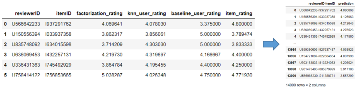
Given a set of (reviewer, item) pairs, we are motivated to predict what rating each reviewer will assign to the paired item they have not yet rated. To solve, we experiment with a variety of different models. We use the ensemble method to combine these models into our final prediction solution.
Intuition tells us that reviewers who have historically tended to rate items in a certain range will continue to rate new items in that same range. Inspired by the baseline code, we implement a simple “reviewer average rating” algorithm to assign each reviewer’s average rating as the predicted rating for any future item they review.
Following a similar approach to our first model, we intuit that items will generally be rated in correlation with their quality. We implement a simple “item average rating” algorithm to assign each item’s average rating as the predicted rating for each item regardless of reviewer.
The neighborhood method is a primary area of collaborative filtering that centers on computing relationships between reviewers1. A reviewer’s neighbors are like-minded reviewers who tend to review the same items. We use the k-nearest neighbor approach to establish each reviewer’s (aka active reviewer) neighborhood, then apply a straight-forward averaging algorithm to predict a rating:

To create the ratings matrix required for collaborative filtering, we assign indexes for each reviewer (row) and each item (column). The standard matrix representation of this data requires ~781.4 million values. A condensed sparse row (csr) matrix representation of the same data is ~3900 times smaller, with only one row per review (200,000). Since Scikit-learn’s nearest neighbor learner supports searches on csr matrices, we opt for the less memory intensive solution and convert the data using scipy.sparse.csr_matrix().
In practice we find cosine similarity with K=10 to produce the most accurate results. Increasing K beyond 10 drastically increases prediction time without improving accuracy.
Latent factor models are another primary area of collaborative filtering1. This approach infers factors to characterize both reviewer and item interaction. We use Apple Inc’s open-source library turicreate (via WSL-Ubuntu) to train a FacorizationRecommender model. We limit the number of factors to 4, use the popular stochastic gradient descent solver2, and train on a large portion of the dataset (90%) to produce our most accurate model3. The latent factorization model allows for predictions above the max reviewer rating (5.0). Clipping our final prediction to the max reviewer rating slightly increases our submission accuracy.
While each model we train is slightly more accurate than the provided baseline predictor, merging our models into an evenly weighted ensemble produces our most accurate results on Kaggle:
| Baseline RMSE | Item Avg. RMSE | k-NN RMSE | Factorization RMSE | Ensemble RMSE |
|---|---|---|---|---|
| 1.31082 | 1.31012 | 1.37928 | 1.29671 | 1.13972 |
In this task, we use review text exclusively to determine which category the reviews belong to: men, women, girls, boys or baby. In the training data, the “categories” column of a review contains multiple subcategories the product belongs to. However, since we only care which category in the target list the review belongs to, we flatten the subcategories list and program it to output which target category exists in the list.
With the exception of BERT, all other input representations feed on review text that are lowered, removed of non-alphabetical symbols, numbers and stopwords. In the case of BERT, we keep the stopwords in the review as BERT tokenizer has its own way of removing stopwords. We also experiment with stemming and decide to exclude it from this report as it does not gain anything in terms of performance.
We notice typographical errors (typos) in our samples and assume these are common in the real world. Typos on certain keywords will certainly lower our accuracy in the task. We believe further works in automatic spelling correction during preprocessing will provide non-trivial gain to our current performance.
70% of reviews in the training set are for women's products, followed by reviews for men’s products at 26%. With the majority of training data coming from the women and men categories, our performance certainly varies across different categories and is biased towards women products in new, unseen data.
The longest review has 2,046 words. The median review has 20 words compared to the average length for reviews of 30 words. We chose to keep only the top 2,000 most frequently used words in the corpus and filter the tokens for each review accordingly. True to our intuition, we verify that those less frequent words indeed are not useful in predicting our target category.
Tf-Idf (Term Frequency - Inverse Document Frequency): Tf-Idf is the product of two statistics: term frequency and inverse document frequency. Term frequency is the number of times a term (t) occurred in the document set (d). Inverse document frequency is the logarithmically scaled inverse fraction of the documents that contain the term (obtained by dividing the total number of documents by the number of documents containing the term, and then taking the logarithm of that quotient).
In the project, we use TfidfTransformer from Scikit-learn in tandem with the CountVectorizer as part of the pipeline. In particular, all the reviews in the training set are vectorized into a count matrix that is subsequently transformed into Tf-Idf representation3.
N-grams: Continuing to use the Tf-Idf representation above, we add bigrams and trigrams into the representation. In particular, TfidfVectorizer from Scikit-learn library combined the two steps mentioned in the Tf-idf section above and generated bigrams and trigrams from the reviews4. The purpose of using n-grams is to incorporate word sequence order into the representation.
BiLSTM (Bidirectional Long Short Term Memory): BiLSTM is an extension of RNN architecture (recurrent neural network), a solution class within deep learning. BiLSTM trained two instead of one LSTMs on the input sequence5. The first on the input sequence as-is and the second on a reversed copy of the input sequence. This can provide additional context to the network and result in fuller learning compared to N-grams.
We rely on Keras from Google Tensorflow to implement this representation. Because of the size of the dataset and ultimately the number of trainable parameters (~500k) in the network, we resort to using Google Colab TPU to both train and test for this task. The memory required during the training simply exceeds the hardware that our local laptops provide.
BERT (Bidirectional Encoders Representation from Transformers): BERT is a breakthrough in language modeling because of its use of bidirectional training of Transformer, a popular attention model6. This contrasts to previous efforts in LSTM or BiLSTM, which look at a text sequence either from left to right or combined left-to-right and right-to-left training. A pre-trained BERT model can be fine-tuned to a wide range of language tasks.
We use a pre-trained BERT model from Google Tensorflow for this implementation. The vocabulary used to train this model comes from the Wikipedia and BooksCorpus dataset.
| Tf-Idf (Acc) | N-grams (Acc) | BiLSTM (Acc) | BERT (Loss-Acc) | |
|---|---|---|---|---|
| Logistic Regression | Train: 0.87, Test: 0.84 | Train: 0.99, Test: 0.83 | ||
| MLP | Train: 0.819, Test: 0.816 | Train: 0.23, Test:0.864 |
In this task, we solely rely on the reviewerID and itemID fields. For the set of 200,000 unique reviewer-item columns, we add a “Purchased” column and set it equal to 1, denoting a purchase was made. Given that there are several unique reviewer-item pairs that were not purchased, we opt to create a sparse matrix to represent user-item pairs that were not purchased (0’s), as well as those that were purchased (1’s). The sparse matrix avoids memory issues and allows us to be efficient, as it only saves the locations of reviewer-item pairs that were purchased.
In contrast the ratings prediction task, which involves explicit user feedback, the purchase prediction task involves implicit feedback. A popular method for collaborative filtering when working with implicit data is alternating least squares (ALS). As opposed to solving matrix factorization using SVD (singular value decomposition), ALS is a popular method when working with a large matrix by approximating latent feature vectors for users and items9. Each vector is solved iteratively, with one vector being solved at a time, until convergence.
The implicit.als.AlternatingLeastSquares model from the implicit library10 is used for this task. Given that this is a recommendation model, the values in the prediction vector for each user-item pair are not binary. Rather, the predictions represent the confidence that a user purchased a particular item, with a higher value representing greater confidence that a user purchased an item. Because of this, we convert predictions to binary values based on different threshold values and evaluate which threshold yields the best results.
The ALS model takes in the following hyperparameters: number of latent factors, regularization constant, number of iterations, alpha value (scaling factor that indicates the level of confidence in preference). These are tuned with the training data, with the evaluation metric being area under the curve (AUC). This metric is selected because the prediction values are a range of numbers, whereas the ground-truth values are binary values.
We tested different threshold values to convert predictions to binary values. For example, the top 20% of prediction values for each user are converted to 1’s and the remaining values are converted to 0’s. This is Method 1 in the table below. These converted values are compared against the ground-truth values on mean precision and mean recall. These evaluation metrics are selected, as opposed to accuracy, because the dataset is highly imbalanced, which would naturally yield a decent accuracy. Precision and recall gives a better understanding of model performance, and similar to AUC, these metrics are calculated for each user, then the mean is calculated across all users. The table below summarizes various techniques used to improve model performance after tuning hyperparameters.
80-20 Training-Testing Data Split
| Prediction values converted to 1's | Training Mean AUC | Testing Mean AUC | Testing Mean Precision | Training Mean Recall | Accuracy on Kaggle | |
| Method 1 (M1) | Top 20% of predictions | 0.84186 | 0.72412 | 0.01324 | 0.86977 | 0.67150 |
| Method 2 (M2) | M1 & prediction >= avg. prediction value across all users | 0.83855 | 0.72372 | 0.01447 | 0.89476 | 0.67571 |
| Method 3 (M3) | M2 & new users in Kaggle file assigned value based on item popularity (top 3000 items) | 0.83977 | 0.72345 | 0.01358 | 0.86963 | 0.67692 |
| Method 4 (M4) | M3 & removing users and items with less than 3 interactions | 0.84000 | 0.73157 | 0.00319 | 0.87399 | 0.66642 |
| Method 5 (M5) | M3 & item popularity (top 3000 items) | 0.84236 | 0.80375 | 0.00076 | 0.79717 | 0.67314 |
- Koren et al. 2009 Koren, Yehuda, Robert Bell and Chris Volinsky. “Matrix Factorization Techniques for Recommender Systems.” Computer Volume: 42, Issue: 8 (2009): 30-37.
- Bottou, 2012 Leon Bottou, “Stochastic Gradient Tricks,” Neural Networks, Tricks of the Trade, Reloaded, 430–445, Lecture Notes in Computer Science (LNCS 7700), Springer, 2012.
- https://apple.github.io/turicreate/docs/api/index.html
- https://scikit-learn.org/stable/modules/generated/sklearn.feature_extraction.text.TfidfTransformer.html
- https://scikit-learn.org/stable/modules/generated/sklearn.feature_extraction.text.TfidfVectorizer.html
- https://towardsdatascience.com/sentence-classification-using-bi-lstm-b74151ffa565
- https://github.com/google-research/bert 7.https://colab.research.google.com/github/google-research/bert/blob/master/predicting_movie_reviews_with_bert_on_tf_hub.ipynb
- Y. Hu, Y. Koren and C. Volinsky, "Collaborative Filtering for Implicit Feedback Datasets," 2008 Eighth IEEE International Conference on Data Mining, Pisa, 2008, pp. 263-272, doi: 10.1109/ICDM.2008.22.
- https://implicit.readthedocs.io/en/latest/als.html