Parallel Voronoi

Introduction

My final year programming project for university, for the unit Advanced programming.

The Brief

You are required to identify and evaluate performance gains in a substantial software engineering project by applying advanced programming techniques (such as parallel programming, CUDA, OpenMPI) to a suitable serial programming project.

My Project

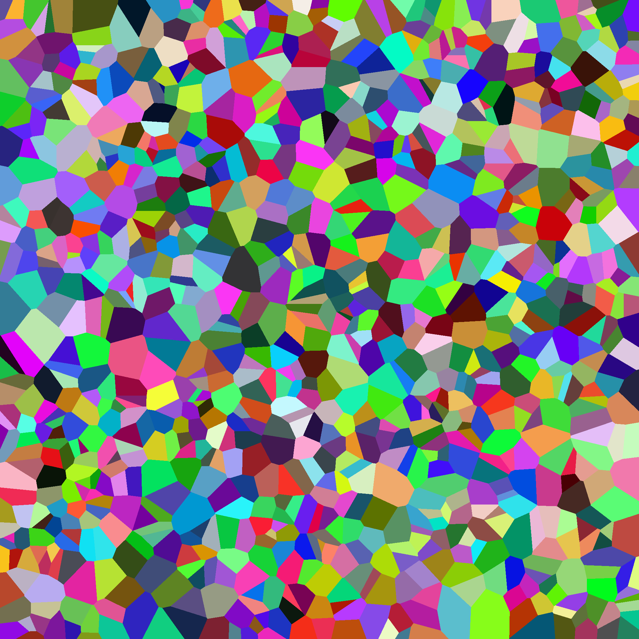
This project implements a simple voronoi map generation algorithm on the CPU in serial then again on the GPU in parallel using CUDA to improve performance. I chose Voronoi as the core algorithm is simple, allowing me to experiment with different parallel techniques.

Structure

The main project contains several sub projects, I wrote the solver_cpu, solver_gpu and tests sub_projects, the rest is mainly based on this project from one of my peers. I took an earlier version of this code and stripped it down to a boilerplate to work from (as can be seen from my earlier commits). Each sub-project is summarised below:

• application, This contains the code for creating the application and GUI, besides plugging in my specific libraries the code in here isn't mine, I did however create the GUI.
• common, This contains some structural code and a local copy of glm to make it more portable.
• tests, Contains the benchmarks to test the speedups. (summarised below)
• solver_cpu, The serial implementation library.
• solver_gpu, The parallel implementation library.

The two libraries each contain 2 'solvers' for creating diagrams. A so called 'brute' approch that checks all cells, and a 'nearest neighbor' or 'NN' approach that creates a series of sub search spaces to reduce the amount of checks needed. It was done this way as in some cases the process of seperating the space is longer than just checking all cells.

Dependencies

• QT 5, used for image generation, benchmarking and qmake for building
  • (QT creator will make running this project much easier)
• C++11 compiler, the CPU implementation relies heavily on C++11
• GLM, this is included in the Common folder, but needed in any case
• CUDA, Nvidias CUDA is used for all parallelisation,
  • Once you have CUDA installed rebuilding for your specific architecture and file paths will be needed
  • This can be done easily in solver_gpu.pro

Implementation

Algorithm

My implementation uses a pretty simple core algorithm:

Seed random points
Give each point a unique colour
for each pixel:
	find the closest point
    set colour equal to colour of point

It is based on the rosetta code algorithm, although my simple serial implementation is slightly different. It is easy to understand and helped a lot with developing things further.

• ind is the index of the cell we are closest to
• dist is the current shortest distance
• each iteration we check if the next cell is any closer, if so update ind to reflect that
• once the third loop is complete push back the index of the closest cell, to get that colour for rendering

for (uint hh = 0; hh < h; hh++)
    {
        for (uint ww = 0; ww < w; ww++)
        {
            int ind = -1;
            uint dist = INT32_MAX;
            for (size_t it = 0; it < _numCells; it++)
            {
                d = utils::DistanceSqrd(cellPos[it], vec2(ww,hh));
                if (d < dist)
                {
                    dist = d;
                    ind = it;
                }
            }

            if (ind > -1)
                ret.push_back(cellColour[ind]);
        }
    }

Parallelisation

For the 'brute' appoach it was very simple to adapt this algorithm. Instead of looping over each pixel as before, each thread takes charge of a single pixel and then checks the cells to see which it is closest to:

uint idx = blockIdx.x * blockDim.x + threadIdx.x;
uint dist = INT32_MAX;
uint colIDX = -1;
for(uint i = 0; i < _cellCount; i++)
{
	uint x = idx&_w-1;
	uint y = (idx-x)/_w;
	uint d = d_distSquared(x, y, _positions[i], _positions[i+_cellCount]);
	if(d < dist)
	{
		dist = d;
		colIDX = i;
	}
}
_pixelVals[idx] = colIDX;

There is an obvious optimisation to be made here, reducing the size of the loop. To do this we break up the problem into several smaller parts, the 'nearest neighbor' approach.

Nearest Neighbor

Splitting the full domain into sub grids allows for the threads in the main algorithm to have far fewer iterations. For example if we split the domain into 64 sub grids and lets say we have 128 cells, the brute version needs 128 iterations, assuming equal cell distribution a cell with all 8 neighbors only needs to iterate over 18 cells, saving 110 iterations, on a 1k image thats 112640 saved iterations!

To do this we generate the points as before, however there are a few added steps. First we complete a point hash, this entails determining which of the sub-grids the cell's centre is in. Once we have this, we calculate the occupancy of each of these sub grids (i.e. how many cell centres are in each).

With this in mind we sort the cell centre positions based on their hash value, this is done using a zip iterator in thrust, as below:

auto tuple = thrust::make_tuple(d_cellXPositions.begin(), d_cellYPositions.begin());
auto zipit = thrust::make_zip_iterator(tuple);
thrust::sort_by_key(d_hash.begin(), d_hash.end(), zipit);

This basically sorts the hash values, and performs the same swaps to the corresponding cell positions. We then perform an exclusive scan on the sub grid occupancies, this tells us the starting indicies in the cell position vector for each sub grid. For example in a 4 sub grid case with 6 cells: if the occupancy is 2,3,1,1 the scan will return 0,2,5,6, this means the positions in the first cell start at index 0, then the next bunch at 2, then 5 then 6. The occupancy tells us the size of each chunk, meaning we know where to start iterating, and after how many iterations we need to stop.

As with all things there is a cost to this, splitting the domain itself into the sub domains requires processing power. We can illustrate this with the same example from before with only 32 cells, each sub grid only has a 50/50 chance to contain a cell, so we need to do ~4 iterations per pixel compared to 32, saving 28 iterations but at the cost of having to fill 3 extra vectors of size 32 and then having to perform operations on them.

BenchMarks

Graph of CPU vs. GPU Benchmarks (5 iterations)

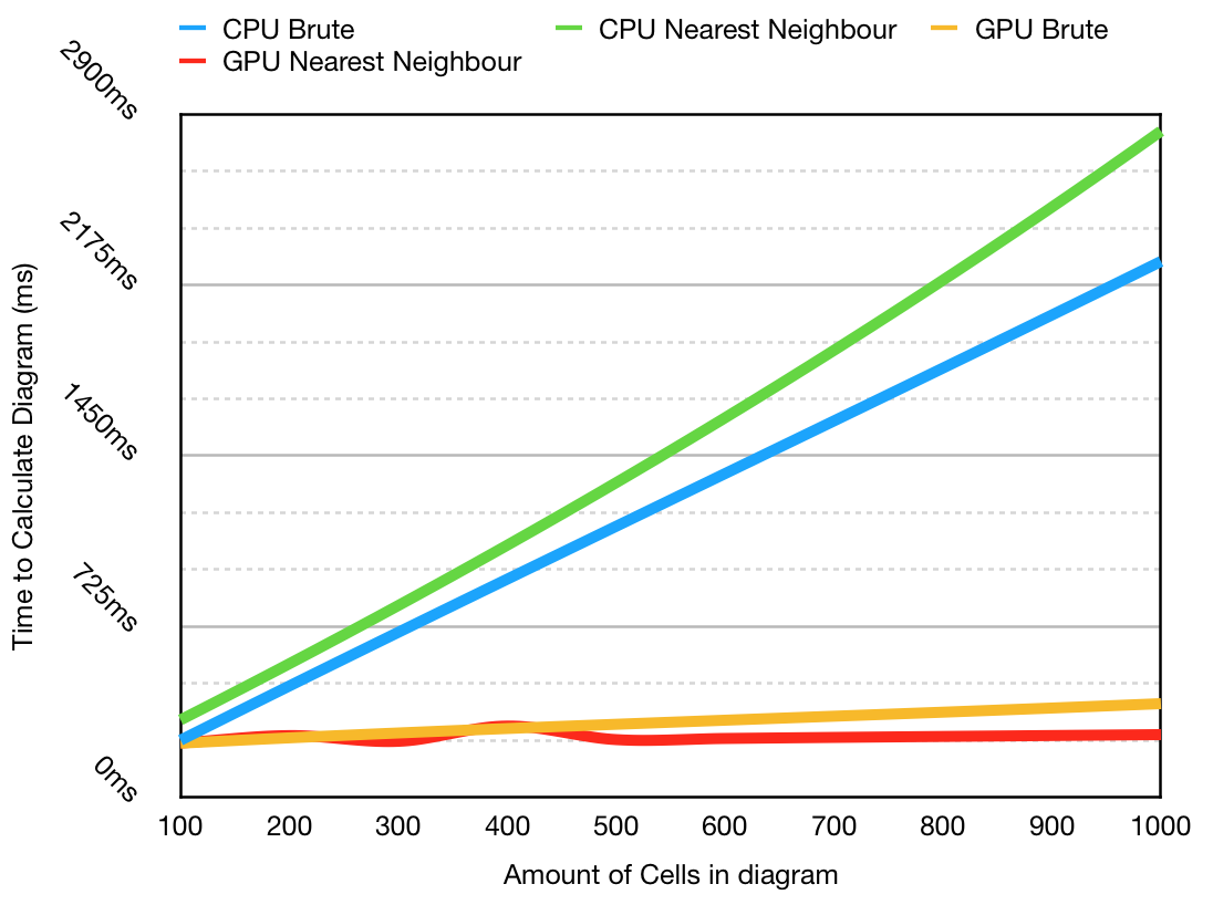
This graph shows that the GPU application is considerably faster as the program scales. The CPU nearest neighbor algorithm is slower in all cases, but this is likely due to the fact that it is implemented using a multimap, compared to a faster array only approach. This is not a perfect comparison, however you can see clearly in the early stages that it illustrates the fixed gap as the hashing function takes time to complete.

Graph of GPU Benchmarks (20 iterations)

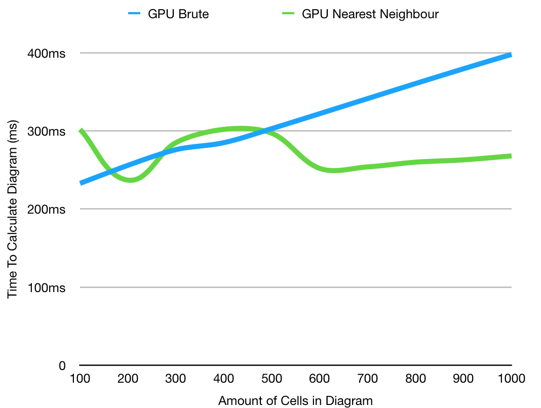
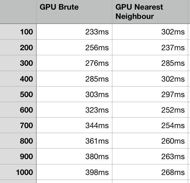
This graph shows only the GPU comparisons, with more iterations, there is an interesting relationship at lower values as the cost of crating the hash tables takes more time than just checking each of the cells, as discussed above. The fact they overtake each other a few separate times is likely due to external factors. The take away is therefore that in general using the brute diagram is rarely advantageous, and therefore using the nearest neighbor version is preferential.

Future Work

There are some errors in the nearest neighbor GPU diagrams, the can sometimes iterate over too few cells, or there is a clamping effect near the edges, as seen below:

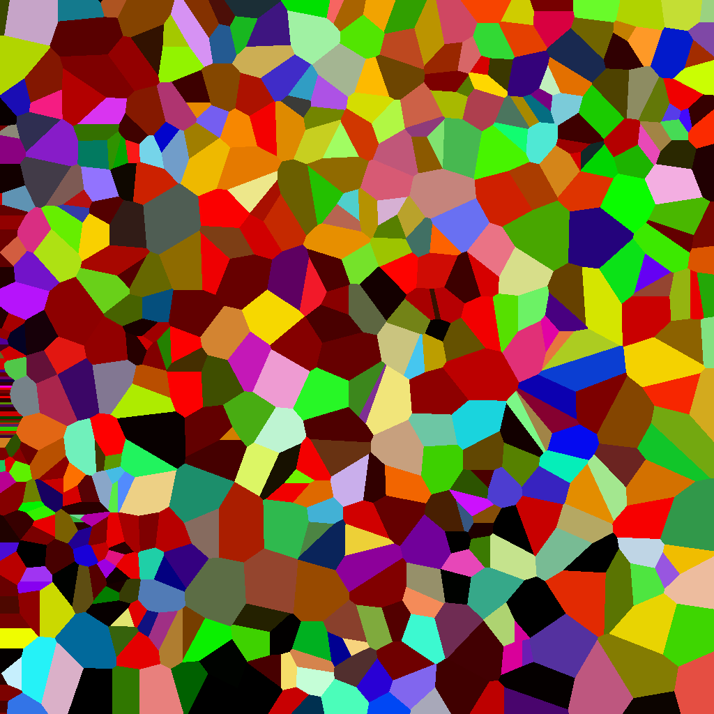
This is the first priority to fix, however it was not possible in the timeframe of the project.

The image name box doesn't work as intended and all images are named export.png, this is not really a problem but might want to be changed in future.