a R project of manipulating and fitting data into regression
This report is to build and select a model for the response y, using the generated data set "dat.cvs" given by the course instructor. Most of the tools studied in course STAT 5120 (Linear Regression) will be used to facilitate model selection, model estimation, model validation, and model diagnosis procedures. The code and report are written by Shaoran Sun individually.
Data: Data contains one response variable, y, and 10 predictors, x1, x2 ... x10. There are 100 instances of data, in total of 100 rows.
Goal: To build and select a model for the response y.
Language: R
               y          x1           x2          x3          x4           x5          x6          x7          x8           x9         x10
1   2.436641e+02  1.08580359  1.114076637  0.45462375  1.69147892  0.106603041  1.90546080 -0.64313318  0.83133738  0.069397226  1.13955430
2   1.348317e+00  1.30488896  1.311393972 -2.01623853 -0.14386029  0.048113406  0.13304981  0.77112214 -1.00337110 -0.637381125  0.36182605
3   2.785373e+00  1.03064839  1.032495758  1.02785284 -0.30580807 -0.689535891 -0.96139722 -0.42695282 -2.03898688 -1.327918885  0.50456596
4   4.870431e+01  0.15783723  0.115275934 -0.12345028  1.71466970  0.726207244  0.13140390  0.34750769  1.62399961 -0.702380618 -0.53134563
5   5.107077e+03  1.32553541  1.270779866 -0.47953329 -1.26886600  1.783569221 -0.38016806 -1.69596388  1.17447004 -0.444843952  0.47327357
6   2.461621e+01  0.17907553  0.169041211  1.10933527 -1.54807478  0.111867633  0.72595169  1.42055461  0.27589284 -0.815191465  2.17941996
7   4.053033e-01 -1.15115545 -1.158052862 -0.26611181 -1.04691094 -0.234039291  0.24481605  0.97600319  1.83334807  0.185934914  1.06412371
8   1.273015e+00  0.34749784  0.413766183 -1.14806766  2.07995485 -0.522305869  0.28911221 -0.90288983  0.16025309 -2.035447258  1.41167025
9   1.750351e+04  1.09237146  1.068349232 -0.31490694  0.78322136  1.674133143  0.23688817 -0.47114442  0.20716043 -0.798898709 -0.46691668
10  1.627548e+05 -0.12377383 -0.101591919  0.14495762 -0.80827415 -0.469902806 -0.58441930 -0.68181262 -0.06050827 -0.629779662  0.55953961
11  1.142597e+04  3.62769114  3.608260193  0.08461995 -2.67794463  0.271191966 -1.28401940 -0.55178324  0.14962121 -0.624638810  1.82517774
12  3.286586e+00  1.30989523  1.307003554  0.14383078 -0.93232006 -1.072868526  1.44455897  1.95752485  0.74129585 -1.516699256  0.18046497
13  1.317835e+01  0.75371880  0.861374750 -0.47295516  0.72538498 -0.417091415  0.28162045  0.71172742  0.45612887  0.713363388  1.64755010
14  7.994837e+01  1.08365898  1.057540228  0.40165760 -2.39403767  0.846814894 -0.67379802  0.40452412 -0.22245711  0.940187027  0.02070462
15  1.254888e+01  0.36798425  0.355010226 -0.91801520 -1.46354593  0.606506960 -0.04757949 -0.34626245  0.68569564 -1.695373745  0.54561368
16  6.475994e+02  0.56864183  0.640659644  0.54047899  0.18522984  1.028743441  0.04754917 -0.16413534  0.21921100  0.364608977  1.21556816
17  1.883914e+02 -1.28581387 -1.212272920  1.48905504 -0.41666222  1.107018328 -0.56406240  0.12190554 -0.36376932 -0.241138967  0.72169162
18  1.435408e-02 -1.26743305 -1.234753509  0.97972598 -0.19470807 -0.760967134 -0.80492656 -0.86978750  0.39825746  1.158414868 -0.30776948
19  2.152715e+03 -1.06712497 -1.084466308  0.53220005  0.22177933  1.829845819 -0.73342870 -0.94666949  0.19451624 -0.905648810 -0.18771025
20  2.748900e+01 -1.38924287 -1.443990181  2.09600223 -0.67593870  0.831477112  0.13696804 -0.05774661 -0.76973991 -0.788922227  1.45771451
- Log Transformation
- Detecting Outliers in Predictors with leverages
- Detecting Influential Observations with DFFITS and Cook's Distance
- Automated Forward Selection Procedure
- Diagnosing Multicollinearity with Variance Inflation Factor (VIF)
- General Linear F Test
*Criteria for statistical significance is P<0.05.

- y is log-transformed
- Entry 10 is removed due to large influence to the overall data
- Predictors x1, x6, x7, x8, x9, and x10 are removed due to insignificance.
- Predictors x2, x3, x4, and x5 are kept, and combined as a first order model.
Call:
lm(formula = y ~ x2 + x3 + x4 + x5)

Residuals:
     Min       1Q   Median       3Q      Max
-2.29129 -0.46534  0.00512  0.62212  1.87873

Coefficients:
            Estimate Std. Error t value Pr(>|t|)
(Intercept)  1.50163    0.09635  15.584  < 2e-16 ***
x2           1.99583    0.08829  22.605  < 2e-16 ***
x3           0.91006    0.10112   8.999 2.46e-14 ***
x4           0.40358    0.08986   4.491 2.01e-05 ***
x5           3.34805    0.09792  34.191  < 2e-16 ***
---
Signif. codes:  0 ‘***’ 0.001 ‘**’ 0.01 ‘*’ 0.05 ‘.’ 0.1 ‘ ’ 1

Residual standard error: 0.9338 on 94 degrees of freedom
Multiple R-squared:  0.955,	Adjusted R-squared:  0.9531
F-statistic: 498.6 on 4 and 94 DF,  p-value: < 2.2e-16
Intercept, x2, and x5 all have p-values of (< 2e-16), x3 has p-value of 2.46e-14, and x4 has p-value of 2.01e-05. The overall p-value is (< 2.2e-16). These p-values are all less than 0.05 and significant.
R-Square is 0.955, which means model represents 95.5% of the data.
I first plot in all 10 variables in responding to y. All the p-values to the variables are greater than 0.05, which indicates that none of the variable is significant.
The 5 assumptions about linear regression are:
- There exists a linear relation between the response and predictor variable(s).
- The error terms have the constant variance
- The error terms are independent, have mean 0.
- Model fits all observations well (no outliers).
- The errors follow a Normal distribution.
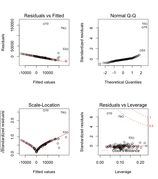
The Residuals vs Fitted graph suggested that residuals do not fall in a horizontal band around 0, and they have an apparent pattern. Assumption 1 and 3 are not met.
The residuals also do not have similar vertical variation across fits. Assumption 2 is not met.
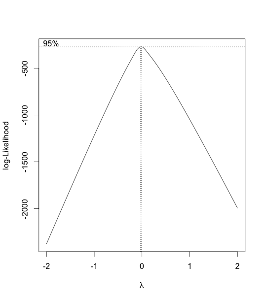
Hence, we consider using a boxcox transformation to test for log-likelihood.
As we can see from the boxcox graph, λ is very close to 0. So we consider a log-transformation.
After the transformation, some of the predictors are starting to become significant, namely, x3, x5, and intercept. The overall p-value also becomes very significant, comparing to before the transformation, where p-value = 0.36.
Coefficients:
             Estimate Std. Error t value Pr(>|t|)
(Intercept)  0.291661   0.094356   3.091  0.00306 **
x1          -1.345198   1.442098  -0.933  0.35479
x2           1.945520   1.438514   1.352  0.18148
x3           0.420027   0.067545   6.219 5.93e-08 ***
x4           0.099419   0.060714   1.638  0.10694
x5           0.960796   0.088476  10.859 1.34e-15 ***
x6           0.025913   0.070012   0.370  0.71264
x7           0.005896   0.075022   0.079  0.93763
x8           0.017321   0.066587   0.260  0.79569
x9           0.120206   0.061508   1.954  0.05549 .
x10         -0.034564   0.073845  -0.468  0.64150
---
Signif. codes:  0 ‘***’ 0.001 ‘**’ 0.01 ‘*’ 0.05 ‘.’ 0.1 ‘ ’ 1

Residual standard error: 0.5092 on 58 degrees of freedom
  (30 observations deleted due to missingness)
Multiple R-squared:  0.7508,	Adjusted R-squared:  0.7079
F-statistic: 17.48 on 10 and 58 DF,  p-value: 4.289e-14
From the above graphs, we can see that outliers definitely exist, possibly, data 10.
Obtain leverages and two measures that can be used to identify influential points, DFFITS (difference in fits) and Cook's Distance.
Influence
*Note that influence of 10th data is way too high
          1           2           3           4           5           6           7           8           9          10*         11          12
 0.36165149 -2.03679604 -1.25990826 -0.87294012 -0.59094408  0.22694916  0.91445506 -0.42747145  0.67615956 12.09277675  0.39684465  0.70673482
         13          14          15          16          17          18          19          20          21          22          23          24
 0.61301290 -1.54270869 -0.57145897 -0.49268510  0.90761831 -1.89567053  1.50472567  0.03107907  0.21320996  0.73273280 -0.66043868  0.39177543
         25          26          27          28          29          30          31          32          33          34          35          36
-0.97302267 -2.12985599  0.39241405 -0.96315529  0.36131924  0.52319298 -0.47421161 -1.21115573  0.28165607 -2.37873048  0.36915979 -0.05378739
         37          38          39          40          41          42          43          44          45          46          47          48
-0.05074383  0.49917022 -0.72100531 -2.16000066  0.24585338  0.43959228  0.97031349  0.04012755  1.02409875 -1.77783334  0.56734973  0.49731647
         49          50          51          52          53          54          55          56          57          58          59          60
 1.64630937 -1.89003794 -0.47072953 -0.26611134 -0.01188162 -0.82421181 -1.06336897 -0.88784144 -0.48258014  0.84599502 -0.66984518 -0.51079971
         61          62          63          64          65          66          67          68          69          70          71          72
 0.22063896 -0.96786752 -0.63538811 -0.24984842 -1.38626689  0.14034692  1.48881825 -0.53317116  0.34388223 -0.04063531 -0.29729509 -0.36282110
         73          74          75          76          77          78          79          80          81          82          83          84
-0.09116264  1.38740278 -0.32815101  1.19629503  0.57524205 -0.71165091  1.82581743 -0.41373586 -0.03320768 -0.36846335 -1.62344667 -0.53836283
         85          86          87          88          89          90          91          92          93          94          95          96
 0.86190740  0.16400262  0.82308678 -0.46164896  1.50089022 -1.98097576  0.40999962  0.34303544  0.28850747  0.16727313 -0.05365871 -0.60549986
         97          98          99         100
-0.52297153  1.18638495  0.02364513  1.10739083
DFFITS
*DFFITS should be less than 1
     10
2.57098
Cook's Distance
*Note that distance of 10th data is also way higher than other data points
    1     2     3     4     5     6     7     8     9    10*   11    12    13    14    15    16    17    18    19    20    21    22    23    24    25
0.001 0.017 0.007 0.003 0.002 0.000 0.003 0.002 0.002 0.209 0.002 0.003 0.002 0.010 0.001 0.001 0.004 0.014 0.010 0.000 0.000 0.007 0.001 0.000 0.003
   26    27    28    29    30    31    32    33    34    35    36    37    38    39    40    41    42    43    44    45    46    47    48    49    50
0.026 0.001 0.004 0.001 0.001 0.003 0.012 0.000 0.018 0.000 0.000 0.000 0.001 0.003 0.026 0.000 0.001 0.006 0.000 0.003 0.011 0.002 0.001 0.026 0.017
   51    52    53    54    55    56    57    58    59    60    61    62    63    64    65    66    67    68    69    70    71    72    73    74    75
0.001 0.000 0.000 0.004 0.011 0.003 0.002 0.003 0.004 0.001 0.000 0.006 0.003 0.000 0.009 0.000 0.005 0.002 0.001 0.000 0.000 0.000 0.000 0.011 0.000
   76    77    78    79    80    81    82    83    84    85    86    87    88    89    90    91    92    93    94    95    96    97    98    99   100
0.006 0.001 0.004 0.016 0.001 0.000 0.000 0.011 0.001 0.002 0.000 0.003 0.001 0.016 0.011 0.001 0.000 0.000 0.000 0.000 0.002 0.000 0.005 0.000 0.006
From the output of influence, DFFITS (difference in fits), and Cook's Distance, we can see that observation 10 is indeed an influential outlier. Hence we remove it.
After removing observation 10, the model fits the data better than before, as we can see in the following output table. Next, we will be choosing which predictors are actually significant.
Coefficients:
             Estimate Std. Error t value Pr(>|t|)
(Intercept)  1.482703   0.103688  14.300  < 2e-16 ***
x1           0.692642   2.042699   0.339    0.735
x2           1.295552   2.039959   0.635    0.527
x3           0.909189   0.103719   8.766 1.25e-13 ***
x4           0.407380   0.093778   4.344 3.73e-05 ***
x5           3.322817   0.103653  32.057  < 2e-16 ***
x6          -0.007948   0.099586  -0.080    0.937
x7           0.130916   0.114019   1.148    0.254
x8           0.070550   0.094905   0.743    0.459
x9           0.027593   0.096969   0.285    0.777
x10          0.052156   0.105381   0.495    0.622
---
Signif. codes:  0 ‘***’ 0.001 ‘**’ 0.01 ‘*’ 0.05 ‘.’ 0.1 ‘ ’ 1

Residual standard error: 0.9533 on 88 degrees of freedom
Multiple R-squared:  0.9561,	Adjusted R-squared:  0.9511
F-statistic: 191.6 on 10 and 88 DF,  p-value: < 2.2e-16
We can see that x1 and x2 are highly correlated with 0.999 correlation, and 515 VIFs, which is way greater than 10, the threshold.
We will next apply automated search to search for significant predictors. If x1 and x2 are both in the result, we will remove one of them in the final predictors.
         y     x1     x2     x3     x4     x5     x6     x7     x8     x9    x10
y    1.000  0.554  0.555  0.324  0.042  0.808 -0.015  0.141  0.205 -0.096  0.033
x1   0.554  1.000  0.999  0.060 -0.020  0.063  0.001 -0.003  0.077 -0.085  0.158
x2   0.555  0.999  1.000  0.060 -0.020  0.064  0.003  0.008  0.079 -0.088  0.160
x3   0.324  0.060  0.060  1.000 -0.003  0.126  0.028  0.063  0.017 -0.007 -0.069
x4   0.042 -0.020 -0.020 -0.003  1.000 -0.061  0.000  0.071 -0.144  0.085 -0.112
x5   0.808  0.063  0.064  0.126 -0.061  1.000 -0.030  0.125  0.211 -0.087 -0.042
x6  -0.015  0.001  0.003  0.028  0.000 -0.030  1.000  0.034  0.109 -0.166  0.100
x7   0.141 -0.003  0.008  0.063  0.071  0.125  0.034  1.000  0.019 -0.068 -0.051
x8   0.205  0.077  0.079  0.017 -0.144  0.211  0.109  0.019  1.000  0.044  0.078
x9  -0.096 -0.085 -0.088 -0.007  0.085 -0.087 -0.166 -0.068  0.044  1.000 -0.058
x10  0.033  0.158  0.160 -0.069 -0.112 -0.042  0.100 -0.051  0.078 -0.058  1.000
Now I use automated search, after removing data 10 from the data set.
Using automated forward search, we get x2, x3, x4, and x5 are chosen, among which all are significant with p-values way less than 0.05. The overall fitting of the 4 predictors results in a p-value of (< 2.2e-16). This proves that after log-transformation, removing data 10 and automated forward selection, the model fits better. x1 and x2 are NOT both in the result, so there is no multicollinearity issue.
Coefficients:
            Estimate Std. Error t value Pr(>|t|)
(Intercept)  1.50163    0.09635  15.584  < 2e-16 ***
x5           3.34805    0.09792  34.191  < 2e-16 ***
x2           1.99583    0.08829  22.605  < 2e-16 ***
x3           0.91006    0.10112   8.999 2.46e-14 ***
x4           0.40358    0.08986   4.491 2.01e-05 ***
---
Signif. codes:  0 ‘***’ 0.001 ‘**’ 0.01 ‘*’ 0.05 ‘.’ 0.1 ‘ ’ 1

Residual standard error: 0.9338 on 94 degrees of freedom
Multiple R-squared:  0.955,	Adjusted R-squared:  0.9531
F-statistic: 498.6 on 4 and 94 DF,  p-value: < 2.2e-16
Next, we will use techniques in Model Comparison and Selection, by comparing R2.adj, PRESS, AIC, BIC, and Cp. We will be using data after removing outlier and log-transformation.
> ###############################
> ##Find model with best R2.adj##
> ###############################
>
> i<-R2.adj == max(R2.adj) ##what index has the maximum R2.adj
> (1:2^10)[i] ##2^10 because 10 potential predictors
[1] 489
> round(results[i,],3)
     p     R2 R2.adj  PRESS    AIC    BIC     Cp
 6.000  0.956  0.953 92.026 -7.954  7.617  2.057
>
> models[i,]
   x1    x2    x3    x4    x5    x6    x7    x8    x9   x10
FALSE  TRUE  TRUE  TRUE  TRUE FALSE  TRUE FALSE FALSE FALSE
>
> ############################################
> ##Find model with best PRESS, AIC, BIC, Cp##
> ############################################
>
> i2<-PRESS == min(PRESS) ##what index has the min PRESS
> (1:2^10)[i2] ##2^10 because 10 potential predictors
[1] 481
>
> i3<-AIC == min(AIC) ##what index has the min AIC
> (1:2^10)[i3] ##2^10 because 10 potential predictors
[1] 481
>
> i4<-BIC == min(BIC) ##what index has the min BIC
> (1:2^10)[i4] ##2^10 because 10 potential predictors
[1] 481
>
> i5<-Cp == min(Cp) ##what index has the min Cp
> (1:2^10)[i5] ##2^10 because 10 potential predictors
[1] 481
>
>
> models[i2,]
   x1    x2    x3    x4    x5    x6    x7    x8    x9   x10
FALSE  TRUE  TRUE  TRUE  TRUE FALSE FALSE FALSE FALSE FALSE
> models[i3,]
   x1    x2    x3    x4    x5    x6    x7    x8    x9   x10
FALSE  TRUE  TRUE  TRUE  TRUE FALSE FALSE FALSE FALSE FALSE
> models[i4,]
   x1    x2    x3    x4    x5    x6    x7    x8    x9   x10
FALSE  TRUE  TRUE  TRUE  TRUE FALSE FALSE FALSE FALSE FALSE
> models[i5,]
   x1    x2    x3    x4    x5    x6    x7    x8    x9   x10
FALSE  TRUE  TRUE  TRUE  TRUE FALSE FALSE FALSE FALSE FALSE
>
> ###########################################
> ##plot the residual against fitted values##
> ###########################################
>
> dat489.lm=lm(y ~ x2+x3+x4+x5+x7)
> summary(dat489.lm)

Call:
lm(formula = y ~ x2 + x3 + x4 + x5 + x7)

Residuals:
     Min       1Q   Median       3Q      Max
-2.28020 -0.41751  0.06503  0.60385  1.93313

Coefficients:
            Estimate Std. Error t value Pr(>|t|)
(Intercept)  1.49739    0.09634  15.543  < 2e-16 ***
x2           1.99599    0.08820  22.629  < 2e-16 ***
x3           0.90480    0.10114   8.946 3.47e-14 ***
x4           0.39580    0.09006   4.395 2.94e-05 ***
x5           3.33487    0.09857  33.832  < 2e-16 ***
x7           0.11749    0.10791   1.089    0.279
---
Signif. codes:  0 ‘***’ 0.001 ‘**’ 0.01 ‘*’ 0.05 ‘.’ 0.1 ‘ ’ 1

Residual standard error: 0.9328 on 93 degrees of freedom
Multiple R-squared:  0.9556,	Adjusted R-squared:  0.9532
F-statistic: 399.9 on 5 and 93 DF,  p-value: < 2.2e-16

>
> dat481.lm=lm(y ~ x2+x3+x4+x5)
> summary(dat481.lm)

Call:
lm(formula = y ~ x2 + x3 + x4 + x5)

Residuals:
     Min       1Q   Median       3Q      Max
-2.29129 -0.46534  0.00512  0.62212  1.87873

Coefficients:
            Estimate Std. Error t value Pr(>|t|)
(Intercept)  1.50163    0.09635  15.584  < 2e-16 ***
x2           1.99583    0.08829  22.605  < 2e-16 ***
x3           0.91006    0.10112   8.999 2.46e-14 ***
x4           0.40358    0.08986   4.491 2.01e-05 ***
x5           3.34805    0.09792  34.191  < 2e-16 ***
---
Signif. codes:  0 ‘***’ 0.001 ‘**’ 0.01 ‘*’ 0.05 ‘.’ 0.1 ‘ ’ 1

Residual standard error: 0.9338 on 94 degrees of freedom
Multiple R-squared:  0.955,	Adjusted R-squared:  0.9531
F-statistic: 498.6 on 4 and 94 DF,  p-value: < 2.2e-16
####Step 8: General F-test Model 481 is a reduced model of 489, with an extra x7. We apply a General F-test to test if x7 is significant.
Analysis of Variance Table

Model 1: y ~ x2 + x3 + x4 + x5
Model 2: y ~ x2 + x3 + x4 + x5 + x7
  Res.Df    RSS Df Sum of Sq      F Pr(>F)
1     94 81.960
2     93 80.929  1    1.0317 1.1856  0.279
p-value is greater than 0.05. Hence, x7 is not significant, and we only need x2, x3, x4, and x5.
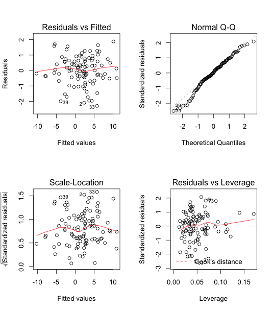
Finally, fit our final model again, and test for goodness of fit.
Call:
lm(formula = y ~ x2 + x3 + x4 + x5)

Residuals:
     Min       1Q   Median       3Q      Max
-2.29129 -0.46534  0.00512  0.62212  1.87873

Coefficients:
            Estimate Std. Error t value Pr(>|t|)
(Intercept)  1.50163    0.09635  15.584  < 2e-16 ***
x2           1.99583    0.08829  22.605  < 2e-16 ***
x3           0.91006    0.10112   8.999 2.46e-14 ***
x4           0.40358    0.08986   4.491 2.01e-05 ***
x5           3.34805    0.09792  34.191  < 2e-16 ***
---
Signif. codes:  0 ‘***’ 0.001 ‘**’ 0.01 ‘*’ 0.05 ‘.’ 0.1 ‘ ’ 1

Residual standard error: 0.9338 on 94 degrees of freedom
Multiple R-squared:  0.955,	Adjusted R-squared:  0.9531
F-statistic: 498.6 on 4 and 94 DF,  p-value: < 2.2e-16
With the given data set "dat.cvs",
- y is log-transformed
- Entry 10 is removed due to large influence to the overall data
- Predictors x1, x6, x7, x8, x9, and x10 are removed due to insignificance.
- Predictors x2, x3, x4, and x5 are kept, and combined as a first order model.
The final model is
| Predictor | P-value |
|---|---|
| intercept | (< 2e-16) |
| x2 | (< 2e-16) |
| x3 | 2.46e-14 |
| x4 | 2.01e-05 |
| x5 | (< 2e-16) |
| overall | (< 2.2e-16) |
All of the above p-values are less than 0.05 and significant.
R-Square is 0.955, which means model represents 95.5% of the data. Model fits the data very well.