
- Introduction
- Stochastic Gradient Descent From Scratch
- Logistic Regression From Scratch
- Kmeans and Kmeans++ From Scratch
- Principal Component Analysis (PCA) From Scratch
In the current landscape, numerous packages and libraries are readily available in the market to enhance productivity in the fields of Data Science, Machine Learning, and Data Analysis. However, it is common for users to adopt these tools without gaining a comprehensive understanding of the underlying algorithms, leading to suboptimal outcomes. Therefore, this repository was created with the objective of delving into key machine learning algorithms, exploring their fundamental concepts and true algorithms, and conducting comparative analyses with existing packages to ensure a better understanding of their functionality and correctness.
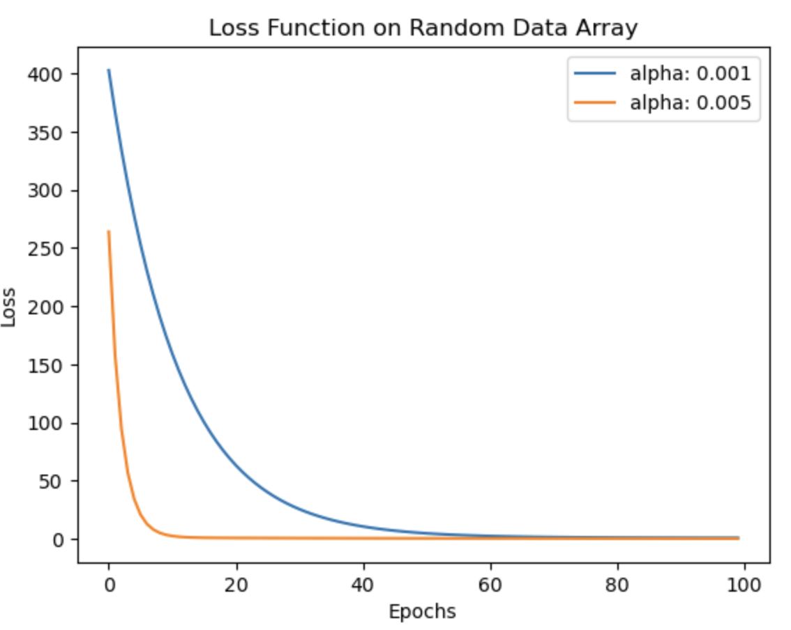
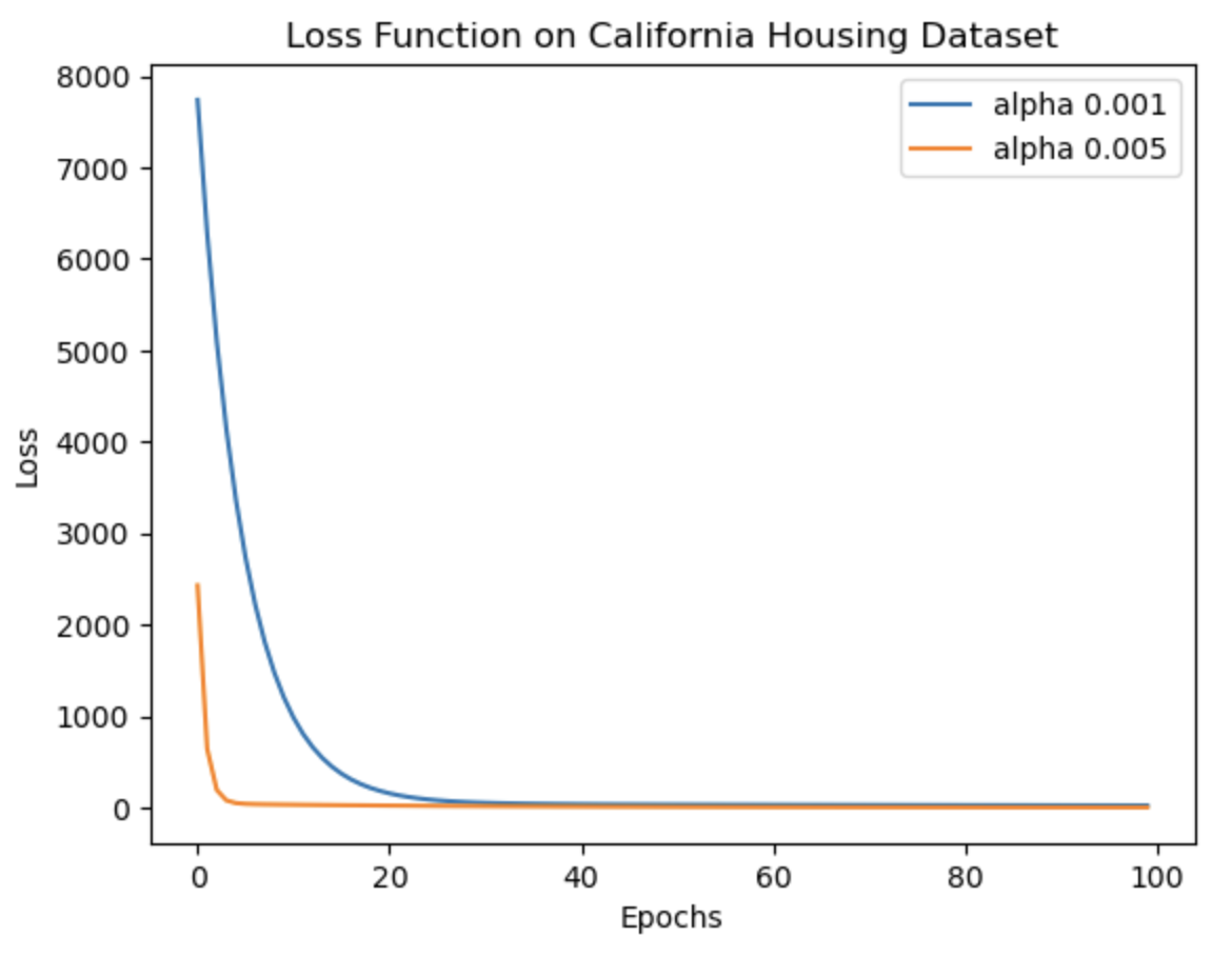
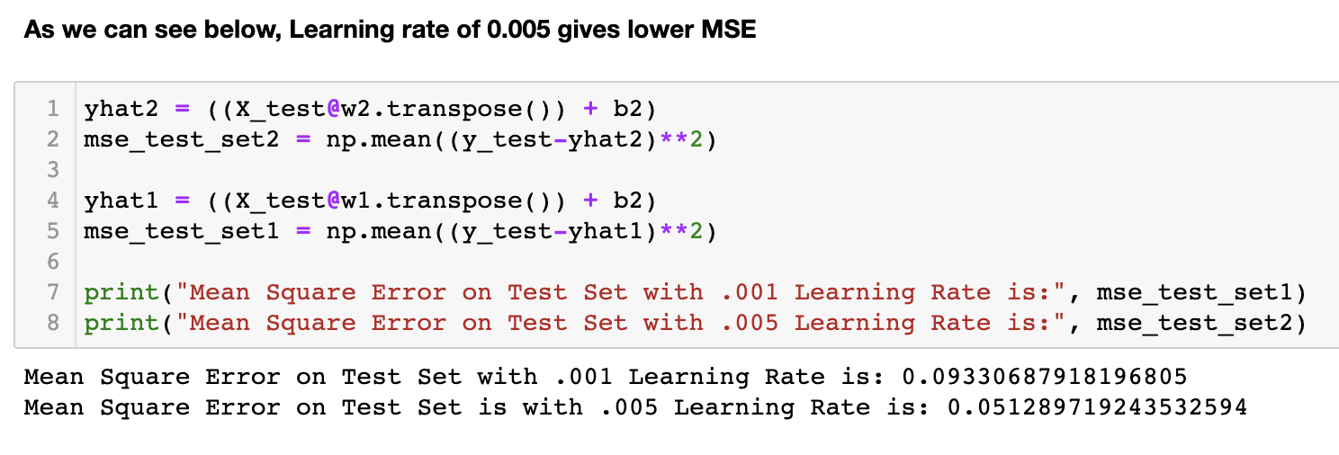
Gradient descent is a fundamental algorithm in almost every application of machine learning. It plays a crucial role in minimizing the error between predicted and ground truth values, forming the foundation of machine learning as we know it today. This notebook focuses on implementing the gradient descent theory and loss function calculations. Initially, these functions are applied to a random data array, followed by their application to the well-known 'California Housing Dataset'. The accompanying images depict the reduction in loss over iterations. Notably, as the learning rate (lr) decreases, the algorithm takes longer to converge and sometimes possibly increases the likelihood of overfitting (thus more MSE on test data with lr 0.001). To validate the implementation, the functions are compared with the scikit-learn SGDRegressor, and it is observed that the results are quite similar. The comparison results are mentioned in detail in the notebook.
Link To Notebook: Stochastic_Gradient_Descent_Scratch.ipynb
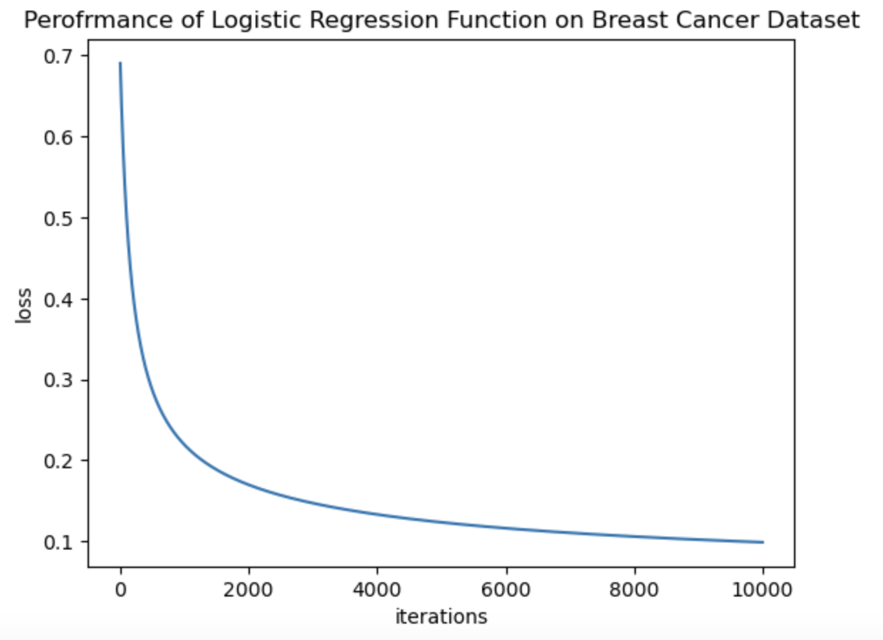
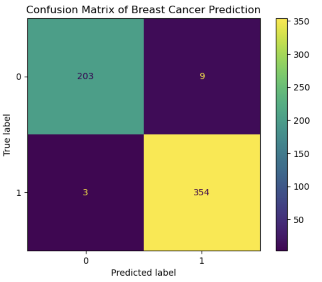
The logistic regression algorithm is a fundamental method for binary classification in machine learning. The concept of logistic regression is not only used in Machine Learning but also in many deep learning algorithms. The idea is similar to the Stochastic Gradient Descent as we mentioned earlier, except, in Logistic Regression we try to predict the pobability of input data to belong to a certain class. Thus Logistic Regression uses concept of cross-entropy function, which compares the predicted probability with the true class label to minimize the loss and then a sigmoid function which classifies the output. In this notebook, I have implemented gradient descent for logistic regression, cross entropy loss function and sigmoid function from scratch. Then the implemented algorithm is applied on the Breast Cancer Wisconsin Data Set and its performance is evaluated. The following images show the performance of the algorithm through Loss Function Graph and Confusion matrix. Finally in the notebook, I also talk about the interpretation of the weights given by logistic regression which is a bit different than linear regression weights.
Link To Notebook: Logistic_Regression_Scratch.ipynb
Clustering is a fundamental concept in unsupervised machine learning, with K-means algorithm being one of the earliest techniques we encounter. Over time, the K-means algorithm has undergone various improvements to enhance its performance, clustering efficiency, and its ability to handle high-dimensional data. Two well-known versions of this algorithm are K-means and K-means++, which continue to be widely used in various data science applications.
In this notebook, I have implemented both the K-means and K-means++ algorithms from scratch. Subsequently, I applied these algorithms to the well-known Iris dataset to evaluate their performance. One limitation of the K-means algorithm is its sensitivity to the random initialization of cluster centroids, which can result in suboptimal clustering outcomes. On the other hand, the K-means++ algorithm follows a similar overall approach but employs a different method for selecting initial centroids, aiming to place them far apart from each other. This initialization strategy leads to improved clustering results. PCA has been performed on the Iris dataset to have better visualization of the clusters. The number of clusters has been chosen to be four for experimental reasons. Sree plot/Elbow method has not been followed for this purpose.
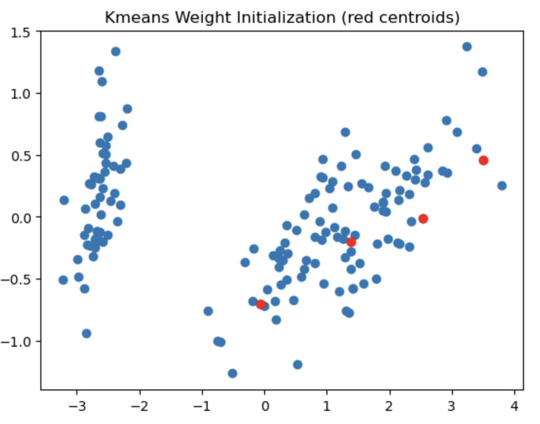
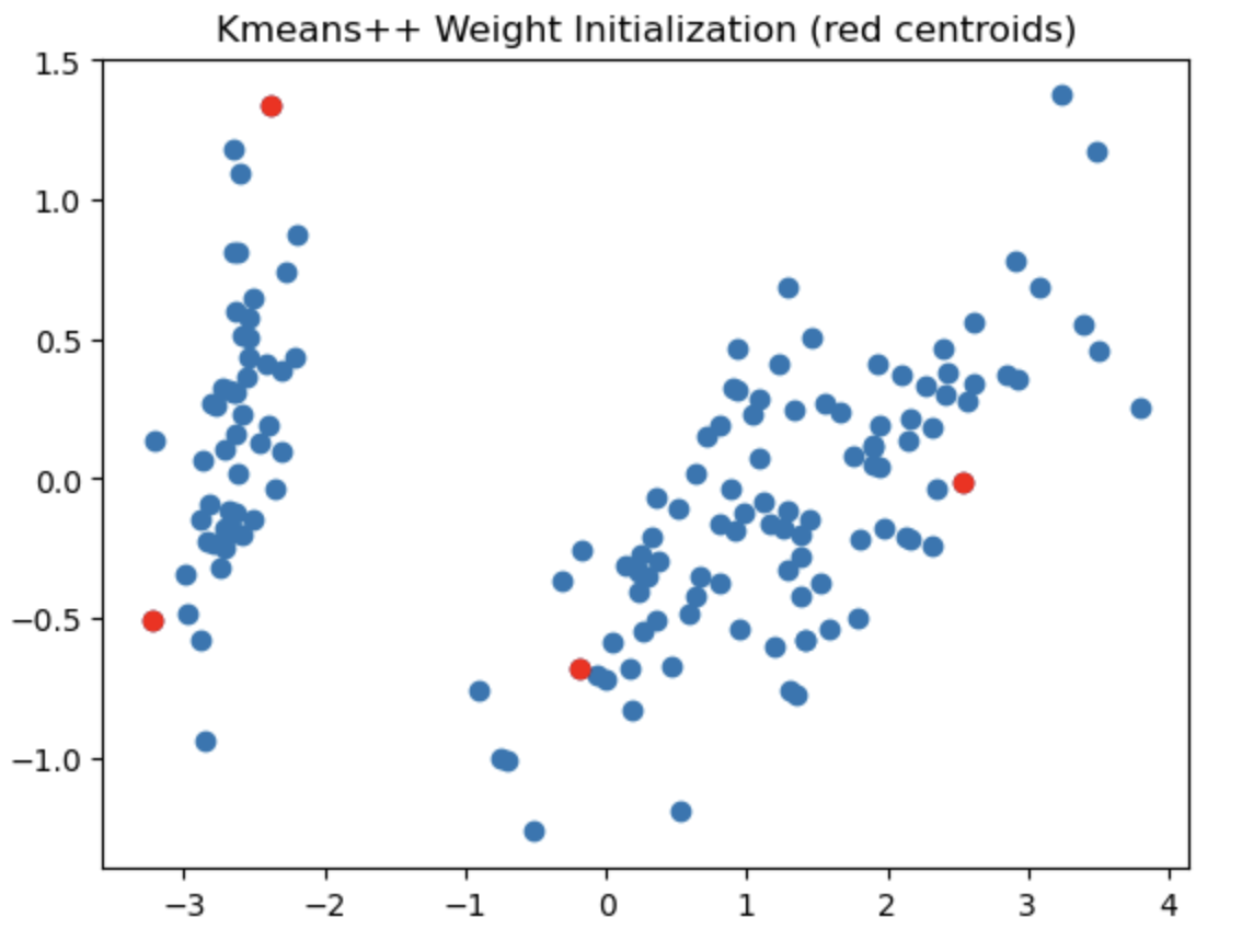
The left most image depicts the shortcomings of Weight Initialization of Kmeans algorithm. The middle image shows how the KMenas++ overcomes that issues. The right most image demonstrates how Kmeans++ algorithm updates the clusters.
Finally to compare performance of the handwritten algorithm I used external dataset and evaluated the clustering result against the sklearn's Kmeans library. I found that both provided almost similar clustering output. Additional details about this dataset and few other facts/thoughts has been discussed inside the notebook.
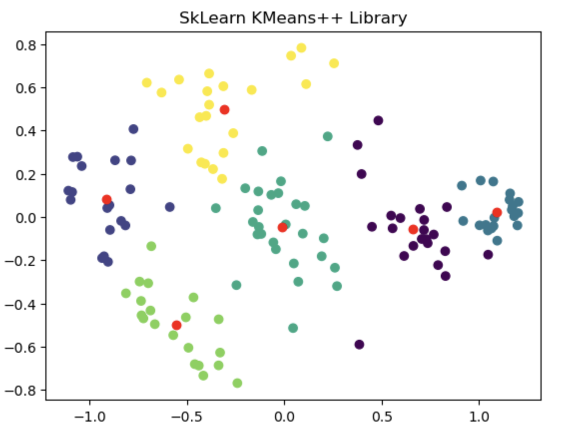
The left image shows the clustering result of the Sklearn library. The right image is where the Kmeans++ manual algorithm is at work.
Link To Notebook: Kmeans & Kmeans++.ipynb
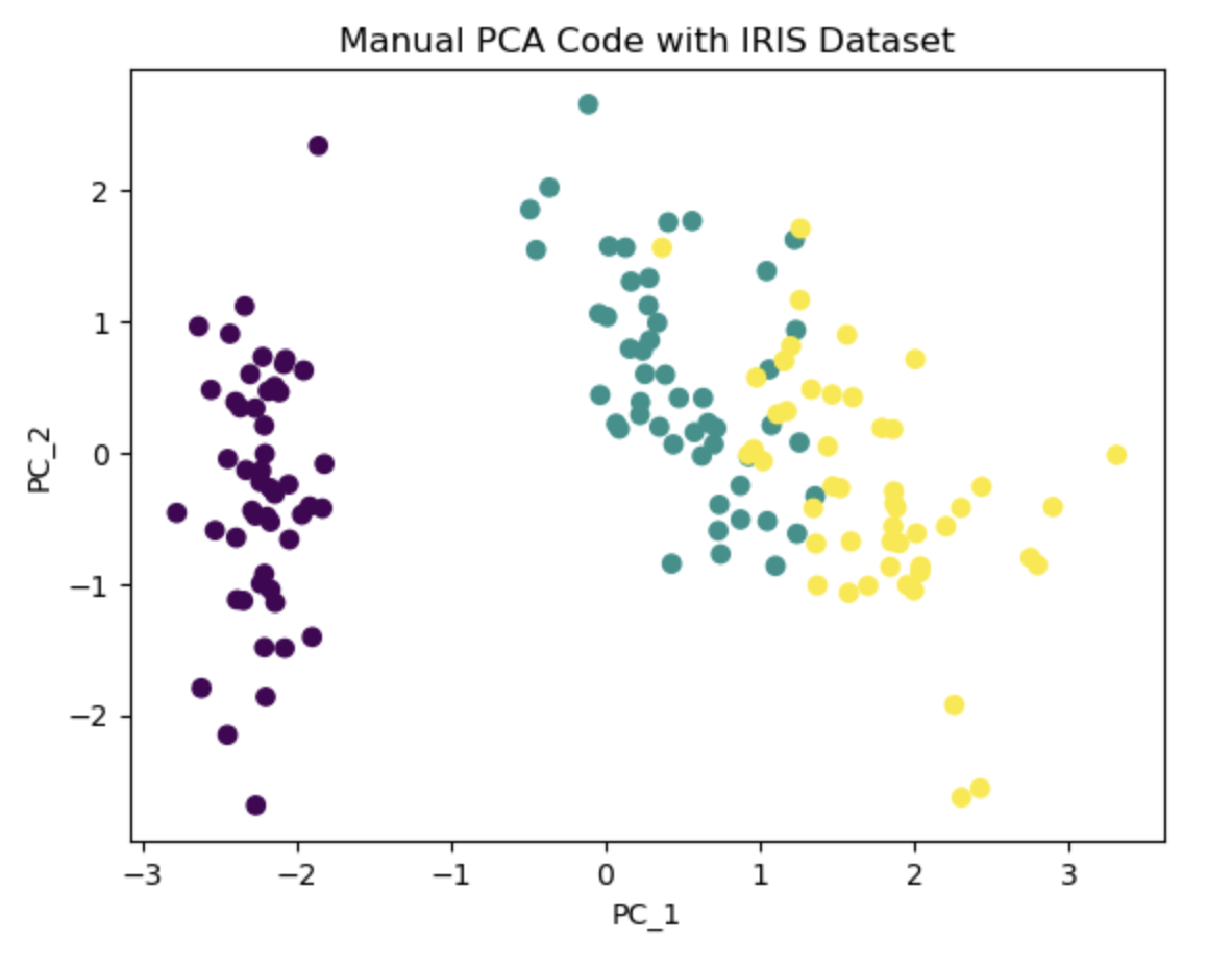
Principal Component Analysis (PCA) is a widely used technique for feature reduction in machine learning. It offers a solution to the Curse of Dimensionality, which arises when there are a large number of features but limited data points available to effectively capture the entire feature space. PCA can also be employed for data visualization in a 2D space.
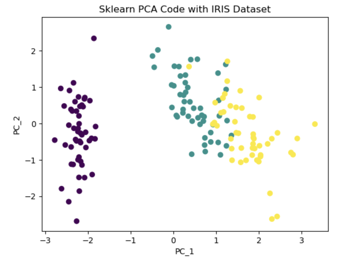
The underlying idea of PCA is to project the features onto axes that capture the maximum variance in the data, enabling a better understanding of the outcome variable. In the PCA algorithm, the first step involves calculating the covariance matrix of the feature space. Subsequently, eigen decomposition is performed to identify the columns corresponding to the highest eigenvalues. Using this information we select the desired number of principal components to retain based on our requirement. These selected components contribute the most to explaining the variance in the data and serve as a reduced set of features for subsequent analysis. In this notebook, I first wrote the PCA algorithm, then used Iris dataset to project its column on a 2-dimensional space for a better visualization. Additionally I used PCA library from Sklearn to compare and validate the results.
Link To Notebook: PCA.ipynb