Special thanks to Sharon Ng (https://github.com/sharonng) for helping me learn the ropes of pandas and seaborn.
I chose the Bob Ross dataset from fivethirtyeight's GitHub repo: https://github.com/fivethirtyeight/data/tree/master/bob-ross
This dataset revolves around Bob Ross' television show, "The Joy of Painting", which aired from 1983 to 1994. Bob Ross painted a total of 381 works while featured guests created an additional 22 paintings for a grand total of 403 paintings over 11 years of airtime.
The creator of this dataset, Walt Hickey, analyzed every episode of Bob Ross' show and generated 67 keywords which described content (trees, water, mountains, clouds, etc.), frame choices, guest artists, and even structures, for a total for 3,224 tags.
I did not read Walt Hickey's analysis until after writing this report.
My initial plan was to understand the following dataset attributes:
- The shape of the dataset:
(403, 69) - What features/attributes were in the dataset: 69 different keywords
- How the dataset was formatted: Categorical, binary-encoded
data_filename = './data/elements-by-episode.csv'
initial_df = pd.read_csv(data_filename)
initial_df.shape()
initial_df.columns
initial_df.head()

--- Output ---
(403, 69)

Index(['EPISODE', 'TITLE', 'APPLE_FRAME', 'AURORA_BOREALIS', 'BARN', 'BEACH',
       'BOAT', 'BRIDGE', 'BUILDING', 'BUSHES', 'CABIN', 'CACTUS',
       'CIRCLE_FRAME', 'CIRRUS', 'CLIFF', 'CLOUDS', 'CONIFER', 'CUMULUS',
       'DECIDUOUS', 'DIANE_ANDRE', 'DOCK', 'DOUBLE_OVAL_FRAME', 'FARM',
       'FENCE', 'FIRE', 'FLORIDA_FRAME', 'FLOWERS', 'FOG', 'FRAMED', 'GRASS',
       'GUEST', 'HALF_CIRCLE_FRAME', 'HALF_OVAL_FRAME', 'HILLS', 'LAKE',
       'LAKES', 'LIGHTHOUSE', 'MILL', 'MOON', 'MOUNTAIN', 'MOUNTAINS', 'NIGHT',
       'OCEAN', 'OVAL_FRAME', 'PALM_TREES', 'PATH', 'PERSON', 'PORTRAIT',
       'RECTANGLE_3D_FRAME', 'RECTANGULAR_FRAME', 'RIVER', 'ROCKS',
       'SEASHELL_FRAME', 'SNOW', 'SNOWY_MOUNTAIN', 'SPLIT_FRAME', 'STEVE_ROSS',
       'STRUCTURE', 'SUN', 'TOMB_FRAME', 'TREE', 'TREES', 'TRIPLE_FRAME',
       'WATERFALL', 'WAVES', 'WINDMILL', 'WINDOW_FRAME', 'WINTER',
       'WOOD_FRAMED'],
      dtype='object')

EPISODE	TITLE	APPLE_FRAME	AURORA_BOREALIS	BARN	BEACH	BOAT	BRIDGE	BUILDING	...
0	S01E01	"A WALK IN THE WOODS"	0	0	0	0	0	0	0	1	...	0	1	1	0	0	0	0	0	0	0
1	S01E02	"MT. MCKINLEY"	0	0	0	0	0	0	0	0	...	0	1	1	0	0	0	0	0	1	0
2	S01E03	"EBONY SUNSET"	0	0	0	0	0	0	0	0	...	0	1	1	0	0	0	0	0	1	0
3	S01E04	"WINTER MIST"	0	0	0	0	0	0	0	1	...	0	1	1	0	0	0	0	0	0	0
4	S01E05	"QUIET STREAM"	0	0	0	0	0	0	0	0	...	0	1	1	0	0	0	0	0	0	0
5 rows × 69 columnsThe next step was to change all of the column names to lowercase so I wouldn't have to abuse my caps lock button throughout this project.
# Change all column names to lowercase
# This will make it easier to group related features in the next section,
# so I don't have to repeatedly toggle caps lock
lowered_df = initial_df.copy()
lowered_df.columns = initial_df.columns.str.lower()Now that the data is slightly easier to read and write, let's sort the features and find out which are most commonly seen throughout Bob's paintings.
-
We're only looking at the paintings' features here, so it's safe to drop the episode and title features.
-
We'll have to transpose the data, meaning swap the axis of the dataset so the rows are indexed by the features and each column is a unique episode.
transposed_df = lowered_df.copy()
transposed_df = transposed_df.drop(labels=['episode', 'title'], axis=1)
transposed_df = transposed_df.transpose()

Transposed dataframe
-
After transposing the dataframe, we can create a new column named "sum" which aggregates each row (painting feature) using the
sumfunction.- This will sum all the 1's in the row to give us a grand total per feature.
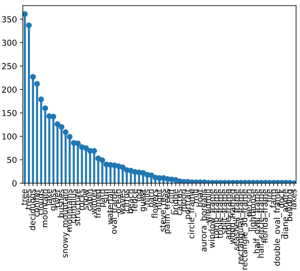
transposed_df['sum'] = transposed_df.agg(func=sum, axis=1)
sum_sorted = transposed_df['sum'].sort_values(ascending=False)
sum_sorted.head(30)

--- Output ---
tree              361
trees             337
deciduous         227
conifer           212
clouds            179
mountain          160
lake              143
grass             142
river             126
bushes            120
snowy_mountain    109
mountains          99
cumulus            86
structure          85
rocks              77
snow               75
cabin              69
winter             69
framed             53
path               49
sun                40
waterfall          39
oval_frame         38
ocean              36
waves              34
cirrus             28
beach              27
fence              24
fog                23
guest              22
Name: sum, dtype: int64
As you can see, Bob Ross loved to draw trees. Below is a bar plot generated with sum_sorted.plot.bar() to show just how much he loved his trees in relation to other features.
- The labels are difficult to read, but we resolve this by grouping features in the Feature Engineering section of this report.
Frequency of each feature
Now that we know that Bob Ross loved to paint trees, let's dial in an see if there's some correlation between the painting's features. We'll use sns.heatmap to generate a correlation heatmap of all features.
- The lighter the pixel, the more positively correlated the two features are
- The darker the pixel, the more negatively correlated the two features are
- NOTE: Not all features are in the axes' labels because it would be crowded and impossible to read. We resolve this later in the Feature Engineering section
# Create correlation heatmap of all ungrouped features
corr = lowered_df.corr()
ax = plt.axes()
ax.set(title='Correlation of all ungrouped features')
sns.heatmap(corr)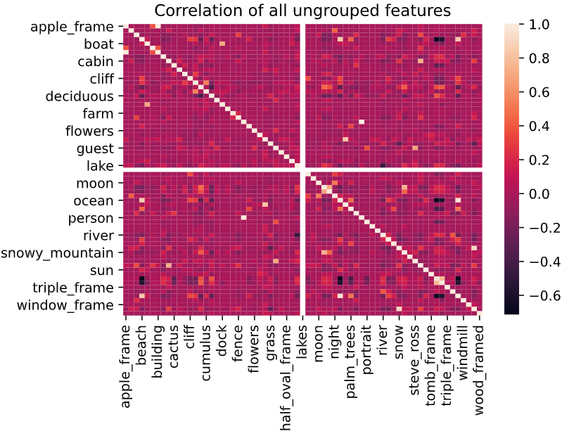
There are a handful of highly positive and negative correlation, let's dive deeper to find what they are
We see in the heatmap that there are a handful of highly positive and negative correlations (look for the very light and dark pixels).
As seen above, we ran into graphical issues when trying to plotting correlations between individual features. Let's group our related features in order to reduce clutter in our plots.
I noticed a lot of the features were related and could be grouped together.
- For example, I could create a group called
group_treeand add the following features:group_tree = ['conifer', 'deciduous', 'palm_trees', 'tree', 'trees'] - Or create a group called
group_structureand add the following features:['barn', 'bridge', 'building', 'cabin', 'dock', 'farm', 'fence', 'lighthouse', 'mill', 'structure', 'windmill']
Grouping these features will allow me to see the bigger picture of how different features are used together.
-
We'll create multiple lists, each a different category containing the related features.
# Group related features, such as trees, structures, water, etc.
group_tree = ['conifer', 'deciduous', 'palm_trees', 'tree', 'trees']
group_structure = ['barn', 'bridge', 'building', 'cabin', 'dock', 'farm', 'fence', 'lighthouse', 'mill', 'structure', 'windmill']
group_water = ['beach', 'lake', 'lakes', 'ocean', 'river', 'waterfall', 'waves']
group_frame = [col for col in lowered_df.columns if 'frame' in col]
group_cloud = ['cirrus', 'clouds', 'cumulus']
group_plant = ['bushes', 'cactus', 'flowers', 'grass']
group_mountain = ['cliff', 'mountain', 'mountains', 'hills', 'snowy_mountain']
group_guest = ['diane_andre', 'guest', 'steve_ross']
group_winter = ['winter', 'snow']

all_groups = group_tree + group_structure + group_water + group_frame + group_cloud + group_plant + group_mountain + group_guest + group_winter
-
Then we'll add all the lists into one list named
all_groups, create thegroup_FEATUREcolumn in the dataframe, and finally drop the individual feature columns from the dataframe in favor of the grouped ones.- NOTE: We're using the
.agg()function again with themaxfunction. This is the same as sayinggroup_cloud = any(['cirrus', 'clouds', 'cumulus'])for each episode. If any of those 3 features == 1, thengroup_cloudwill also == 1.
all_groups_df = lowered_df.copy()
groups = [
    ('group_tree', group_tree), ('group_structure', group_structure),
    ('group_water', group_water), ('group_frame', group_frame),
    ('group_cloud', group_cloud), ('group_plant', group_plant),
    ('group_mountain', group_mountain), ('group_guest', group_guest),
    ('group_winter', group_winter)
]
for group_name, group_columns in sorted(groups):
    all_groups_df[group_name] = all_groups_df[group_columns].agg(func=max, axis=1)
    all_groups_df = all_groups_df.drop(labels=group_columns, axis=1)
- NOTE: We're using the
Our dataframe is now much less cluttered and contains 2/3 fewer columns. We could further group the smaller features together, but I omitted this step because I wanted to show how the less-frequent features related to one another.
all_groups_df

--- Output ---
episode	title	aurora_borealis	boat	fire	fog	moon	night	path	person	...	sun	group_cloud	group_frame	group_guest	group_mountain	group_plant	group_structure	group_tree	group_water	group_winter
0	S01E01	"A WALK IN THE WOODS"	0	0	0	0	0	0	0	0	...	0	0	0	0	0	1	0	1	1	0
1	S01E02	"MT. MCKINLEY"	0	0	0	0	0	0	0	0	...	0	1	0	0	1	0	1	1	0	1
2	S01E03	"EBONY SUNSET"	0	0	0	0	0	0	0	0	...	1	0	0	0	1	0	1	1	0	1
3	S01E04	"WINTER MIST"	0	0	0	0	0	0	0	0	...	0	1	0	0	1	1	0	1	1	0
4	S01E05	"QUIET STREAM"	0	0	0	0	0	0	0	0	...	0	0	0	0	0	0	0	1	1	0
...	...	...	...	...	...	...	...	...	...	...	...	...	...	...	...	...	...	...	...	...	...
398	S31E09	"EVERGREEN VALLEY"	0	0	0	0	0	0	0	0	...	0	0	0	0	1	1	0	1	0	0
399	S31E10	"BALMY BEACH"	0	0	0	0	0	0	0	0	...	0	0	1	0	0	0	0	1	1	0
400	S31E11	"LAKE AT THE RIDGE"	0	0	0	0	0	0	0	0	...	0	1	0	1	1	1	0	1	1	0
401	S31E12	"IN THE MIDST OF WINTER"	0	0	0	1	0	0	1	0	...	0	0	0	0	0	0	1	1	0	1
402	S31E13	"WILDERNESS DAY"	0	0	0	0	0	0	0	0	...	0	0	0	0	1	1	0	1	0	0
403 rows × 22 columnsLet's count the appearances of all features now, including groups:
# Count appearances of all groups
summed_groups_df = all_groups_df.copy()
summed_groups_df = summed_groups_df.transpose().drop(labels=['episode','title'])
summed_groups = summed_groups_df.sum(axis=1).astype(int).sort_values(ascending=False)
summed_groups

--- Output ---
group_tree         369
group_water        303
group_plant        230
group_mountain     183
group_cloud        182
group_structure    102
rocks               77
snow                75
winter              69
group_frame         54
path                49
sun                 40
fog                 23
group_guest         22
night               11
portrait             3
moon                 3
boat                 2
aurora_borealis      2
person               1
fire                 1
dtype: int32
As expected, Bob Ross loved his trees. Over 91% of his paintings contained a tree! But now we also see that he frequently painted water.
Just like before, we can create a simple correlation heatmap and get a more generalized output now that we have groups
all_groups_corr = all_groups_df.corr()
ax = plt.axes()
ax.set(title='Correlation of grouped features')
sns.heatmap(all_groups_corr, yticklabels=True)  # Show every y-axis label instead of every other label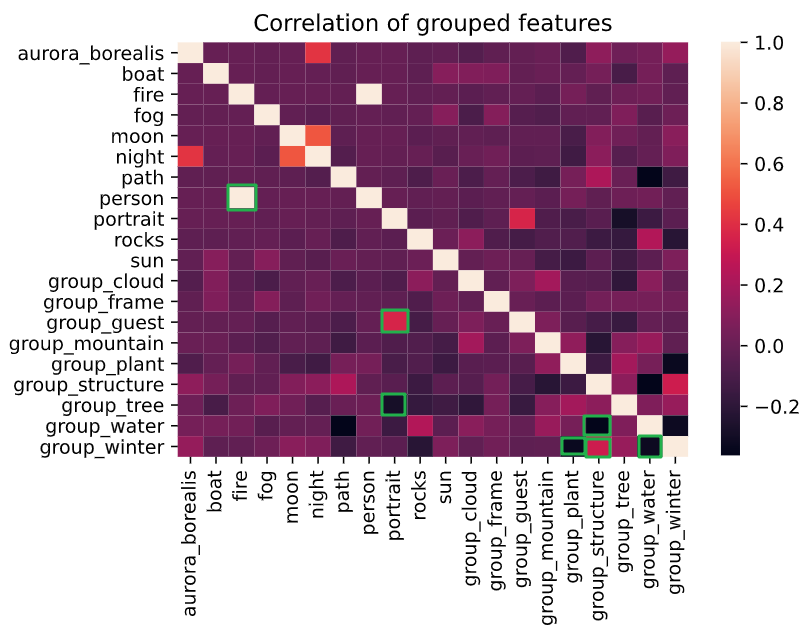
Interesting correlations were highlighted in green boxes
In order to find out which features are highly correlated, we need to refer back to the EDA lab, specifically Question#9 when we were reshaping the data.
-
First we must stack the data. This will change the columns into individual rows. So, instead of have 1 row with 67 columns, we'll have a multi-indexed row with 67 sub-rows with 1 column (correlation %).
corr_high = corr.stack()
corr_high

--- Output ---
apple_frame  apple_frame        1.000000
             aurora_borealis   -0.003522
             barn              -0.010467
             beach             -0.013365
             boat              -0.003522
                                  ...
wood_framed  waves             -0.015140
             windmill          -0.002488
             window_frame      -0.002488
             winter            -0.022669
             wood_framed        1.000000
Length: 4356, dtype: float64
-
Then we'll reset the index, and rename the columns, so we'll have three columns (feature1, feature2, correlation%) and one row for each correlation
corr_high = corr.stack().reset_index().rename(
    columns={'level_0': 'feature1', 'level_1': 'feature2', 0: 'high_corr'}
)
corr_high

--- Output ---

feature1	feature2	high_corr
0	apple_frame	apple_frame	1.000000
1	apple_frame	aurora_borealis	-0.003522
2	apple_frame	barn	-0.010467
3	apple_frame	beach	-0.013365
4	apple_frame	boat	-0.003522
...	...	...	...
4351	wood_framed	waves	-0.015140
4352	wood_framed	windmill	-0.002488
4353	wood_framed	window_frame	-0.002488
4354	wood_framed	winter	-0.022669
4355	wood_framed	wood_framed	1.000000
4356 rows × 3 columns
-
Now that we have all of the correlation values, let's filter the higher correlations and then sort them
- Remember that correlations can be from -1.0 → 1.0. If the absolute value of the correlation == 1.0, then the feature is likely correlating with itself, so we'll have to remove that
corr_high = corr_high[corr_high['high_corr'].abs().between(left=0.5, right=0.99)]
corr_high = corr_high.sort_values(by='high_corr', ascending=False)
# Remove duplicates, every 2nd row is the same as the row above it except feature1/feature2 are swapped
corr_high.iloc[::2, :]

--- Output ---

      feature1	  feature2	          high_corr
2635	ocean	      waves	              0.969188
3364	snow	      winter	            0.916661
237 	beach   	  ocean	              0.855598
4029	waves	      beach	              0.847090
2666	oval_frame	framed	            0.829166
3885	trees	      tree	              0.770751
2427	mountain	  snowy_mountain	    0.750383
3572	structure	  cabin              	0.733814
1192	dock	      boat	              0.706227
3526	steve_ross	guest	              0.697115
2478	mountains	  mountain	          0.691492
1003	cumulus	    clouds              0.546095
2543	night     	moon	              0.516984
4084	waves     	trees	              -0.565289
256 	beach	      trees	              -0.578704
2632	ocean	      trees              	-0.590175
4083	waves      	tree	              -0.685392
255	  beach      	tree	              -0.688180
3801	tree      	ocean	              -0.718906
# More information on `corr_high[corr_high['high_corr'].abs().between(left=0.5, right=0.99)]`

corr_high[corr_high['high_corr'].abs().between(left=0.5, right=0.99)]
# This applies the `abs()` function to the `high_corr` column, so it turns all negative numbers into positive
# `.between(0.5, 0.99)` returns all values between 0.5 and 0.99
From the correlation data, we can gather the following obvious insights:
- When Oceans are painted, there's a positive correlation of Waves also being painted. Make sense.
- When a Beach is painted, there's a positive correlation of an Ocean also being painted. This also makes sense.
We can also gather the following interesting insights:
- When a painting is Framed, it's likely it'll be an Oval Frame.
- When a painting contains Waves, such as an Ocean or Beach painting, it's unlikely for there to be any Trees.
Grouping features has its benefits and drawbacks. In short, correlations become more muddled and vague, but you can see a bigger picture of how all related features (groups) are correlated with other groups.
- Benefits: We can develop a better understanding of the bigger picture of how features are correlated.
- Drawbacks: We lose the feature-specific correlations, such as the positive correlation of Beach/Ocean/Waves features, when features are grouped together.
From the Grouped Feature Correlation Heatmap, we can find a few interesting correlations surrounded with green boxes...
- Person has a nearly 1.0 correlation with fire. Does Bob Ross like to pain people on fire?
- Portraits are (highly) positively correlated with group_guests and negatively correlated with group_trees.
- Structures are negatively correlated when the painting has water-related features, but positively correlated when the painting has winter-related features.
- Furthermore, plant and water-related features are negatively correlated to winter-related features.
Interesting stuff, huh?
We can find the Mean and Median for ungrouped and grouped features in the following code block:
- For ungrouped features, the Mean occurrence is 48 and the Median is 11.
- It's important to remember that this data is heavily right-skewed because Mr. Ross loved to paint trees. Over 369 of the 403 paintings (92%) contained trees!
- For grouped features, the Mean occurrence is 87 and the Median is 45.
- Grouping the features corrected the skewage a little bit... but the Happy Little Trees are eternally dominant in "The Joy of Painting".
We'll use these Mean and Median values later during our Hypothesis testing.
mean_df = lowered_df.copy()
mean_df.set_index(keys='episode', inplace=True)
mean_df.drop(labels='title', inplace=True, axis=1)
# Average number of occurences for each feature == 48.07
average_occur_mean = mean_df.sum().mean()
# Median number of occurences for each feature == 11
average_occur_median = mean_df.sum().median()
# The Mean (48) is skewed beause Bob Ross loves to draw trees, so we're using the Median (11) number of occurrences instead

grouped_mean_df = all_groups_df.copy()
grouped_mean_df.set_index(keys='episode', inplace=True)
grouped_mean_df.drop(labels='title', inplace=True, axis=1)
# Average number of occurences for each grouped feature == 87
average_occur_mean = grouped_mean_df.sum().mean()
# Median number of occurences for each grouped feature == 45
average_occur_median = grouped_mean_df.sum().median()# Hypothesis 1: If I choose a painting with a Mountain, it's statistically more likely to also have Snow
grouped_df = lowered_df.copy()
grouped_df['group_mountain'] = grouped_df[group_mountain].agg(func=max, axis=1)
grouped_df = grouped_df.drop(labels=group_mountain, axis=1)
num_mountain_paintings = grouped_df['group_mountain'].sum() # 183 paintings (45.41%) have a Mountain, above mean and median
grouped_df['snow'].sum() # 75 paintings (18.61%) have Snow, above mean and median (below grouped mean)
grouped_df['snow_with_mountains'] = grouped_df['group_mountain'] & grouped_df['snow']
num_snow_and_mountain = grouped_df['snow_with_mountains'].sum() # 31 paintings have Snow and Mountains, below the mean (48) but above the median (11)
num_snow_and_mountain / num_mountain_paintings # 16.94% of paintings with Mountains also have Snow- Result: This hypothesis was correct!
- In fact, the data shows that only about 17% of all Mountain paintings also contain Snow, whereas only 41% of all Snow paintings also contain a Mountain.
- Furthermore, we can see that the number of paintings that contain a Mountain (183) well exceed the Mean and Median for both ungrouped (48, 11) and grouped (87, 45) feature occurrences.
# Hypothesis 2: If the painting is Framed, it's highly likely the painting will not contain a Tree
grouped_df = lowered_df.copy()
grouped_df['group_tree'] = grouped_df[group_tree].agg(func=max, axis=1)
grouped_df['group_frame'] = grouped_df[group_frames].agg(func=max, axis=1)
grouped_df = grouped_df.drop(labels=group_tree+group_frames, axis=1)

num_all_paintings = len(grouped_df)                      # 403 paintings total
num_framed_paintings = grouped_df['group_frame'].sum()   # 54 Framed paintings
num_framed_paintings / num_all_paintings                 # 13.39% of paintings are Framed

grouped_df['tree_and_frame'] = grouped_df['group_tree'] & grouped_df['group_frame']
num_tree_and_frame = grouped_df['tree_and_frame'].sum()  # 51 Framed paintings with trees
num_tree_and_frame / num_all_paintings                   # 12.66% of paintings are Framed with Trees
num_tree_and_frame / num_framed_paintings # 94.44% of Framed paintings have Trees- Result: This hypothesis was incorrect!
- It turns out that 94% of framed paintings also contain a tree. This is unsurprising after discovering over 91% of Bob's paintings contain a tree.
- No need to compare against the Mean and Median value here.
# Hypothesis 3: If it's a Winter painting, Bob Ross will have also painted a Structure
# Short and neat way to create the same winter_and_structure column as below
all_groups_df[all_groups_df['group_winter'] == 1].loc[   # Bob Ross has 77 Winter paintings (above the mean & median), 19.10% of all paintings
    all_groups_df['group_structure'] == 1].loc[          # of the 77 Winter paintings, 41 contain a Structure (above median) (53.24%)
        all_groups_df['group_guest'] == 0]               # 22 episodes with guests, 5.45% (22/403) of all episodes are guests

grouped_df = lowered_df.copy()
grouped_df['group_winter'] = grouped_df[group_winter].agg(func=max, axis=1)
grouped_df['group_structure'] = grouped_df[group_structure].agg(func=max, axis=1)
grouped_df['group_guest'] = grouped_df[group_guest].agg(func=max, axis=1)

grouped_df = grouped_df.drop(labels=group_winter+group_structure, axis=1)
num_all_paintings = len(grouped_df)
num_winter_paintings = grouped_df['group_winter'].sum()           # 77 Winter paintings
num_structure_paintings = grouped_df['group_structure'].sum()     # 102 paintings with a Structure

num_winter_paintings / num_all_paintings                          # 19.10% of all paintings are Winter-related
num_structure_paintings / num_all_paintings                       # 25.31% of all paintings have a structure

grouped_df['winter_and_structure'] = grouped_df['group_winter'] & grouped_df['group_structure']
# Make sure it's by Bob Ross, not a Guest
grouped_df['winter_and_structure'] = grouped_df['winter_and_structure'].loc[grouped_df['group_guest'] == 0]
num_winter_and_structure = grouped_df['winter_and_structure'].sum()  # 41 Winter paintings by Bob Ross with a Structure
num_winter_and_structure / num_all_paintings                         # 10.42% of paintings are Winter with Structure
num_winter_and_structure / num_winter_paintings # 53.25% of Winter paintings have a Structure- Result: This hypothesis is pointing slightly towards correct, but it's too close to tell.
- There are 41 Winter paintings that contain a Structure.
- This number is lower than the ungrouped Mean of 48 and grouped Mean and Median of (87, 45), so it's unlikely you'll select a Winter painting that also contains a Structure.
- BUT, if you're watching Bob Ross paint a Winter scene, there's a little over 50% chance that he'll also paint a Structure.
- 41 Winter paintings with a Structure is higher than the ungrouped Median of 11. However, I am using grouped features in this hypothesis so it does not make sense to compare the grouped values against ungrouped values.
- This number is lower than the ungrouped Mean of 48 and grouped Mean and Median of (87, 45), so it's unlikely you'll select a Winter painting that also contains a Structure.
Unfortunately, because the dataset is categorical, we are unable to do a true formal significance test.
- This is an oversight on my part. After selecting the dataset, and formulating my hypotheses, I was unaware that you could not normalize skewed categorical data.
- So, instead of performing a significance test, I compared all hypotheses to the Mean and Median values for both ungrouped and grouped features.
The next steps in analyzing this data could include describing how Bob Ross & friends name their paintings based on what features were included. Often, the main feature would also have a keyword in the title.
- For example, if the painting had a lake, it would often include the word "Lake" in the title.
One could analyze how much weight each feature had on the naming scheme of the painting's final title.
The data was categorical, simple, and easy to work with and understand at first glance.
However, after deep diving into some of the features and watching the related "The Joy of Painting" episodes, I noticed a few discrepancies in the features. For example in S03E04, the painting's title is "Winter Night", but the winter label is 0, whereas the snow label is 1.
This led me to question how the dataset's author decided whether a painting included a feature or not. However, it's important to note that discrepancies of this nature are easily resolved by grouping related features.