'promotionImpact' package is for analysis and measurement of promotion effectiveness on a given target variable(e.g. daily sales).
This package provides convenient tools for converting promotion schedule into dummy or smoothed predictor variables and examining the effects of these variables controlled for trend/periodicity/structural change or some prespecified variables(e.g. start of a month).
Just run the code below in R.
install.packages("promotionImpact")
for CRAN version.
Or,
library(devtools)
devtools::install_github("ncsoft/promotionImpact")
for GitHub version.
To install properly, you should install Rtools for your R version at https://cran.r-project.org/bin/windows/Rtools/. Note that when you run the install_github command, you are asked if you want to update other packages. Even if you select 'None', promotionImpact will be installed successfully.
First, you need the following data (Note that promotionImpact contains sample data for practice).
-
Daily target data (e.g., Daily Sales, Daily Active Users(DAU))
-
Promotion schedule data (including Promotion ID, Start/End date and Promotion type)
promotionImpact::sim.data # daily simulated sales data
| dt | simulated_sales |
|---|---|
| 2015-02-11 | 1,601,948,810 |
| 2015-02-12 | 2,048,650,675 |
| 2015-02-13 | 2,288,870,304 |
| ... | ... |
| 2017-09-25 | 1,492,506,224 |
promotionImpact::sim.promotion # simulated promotion schedule data
| pro_id | start_dt | end_dt | tag_info |
|---|---|---|---|
| pro_1_1 | 2015-02-16 | 2015-03-14 | A |
| pro_1_2 | 2015-06-07 | 2015-06-25 | A |
| ... | ... | ... | ... |
| pro_5_10 | 2017-04-02 | 2017-04-26 | E |
Promotions in the sample data were run a total of 50 times during 2015-02-11 ~ 2017-09-25, and 10 times for each of the five types A, B, C, D and E.
The daily sales of the sample data consist of the effects of these promotions, the trend/periodicity factors, the sales surge of the first day of the month(1st day of each month) and some random errors.

The goal is to separate and estimate the effects of each promotion type in the daily sales data.
First, if you want to control the effect of the first day of the month, add the dummy variable of the first day of each month as shown below.
library(dplyr)
sim.data <- sim.data %>%
  dplyr::mutate(month_start = ifelse(substr(as.character(dt),9,10) == '01', 1, 0))
In this way, you can add as many dummy variables as you need to consider when comparing promotional effects.
Now, create the model as shown below.
pri1 <- promotionImpact(data=sim.data, promotion=sim.promotion,
                        time.field = 'dt', target.field = 'simulated_sales',
                        dummy.field = 'month_start',
                        trend = T, period = 30.5, trend.param = 0.02, period.param = 2,
                        logged = TRUE, differencing = TRUE, synergy.promotion = FALSE,
                        synergy.var = NULL, allow.missing = TRUE)
A description of each parameter used above model is given below.
- data : dataset with time.field, target.field and other dummy variables
- promotion : promotion schedule data
- trend : whether a trend exists
- period : If NULL, there is no periodicity. If 'auto', the periodicity is automatically estimated. If you specify a numeric value, the periodicity corresponding to the input number is calculated.
- trend.param : This parameter controls the flexibility of the trend component. The higher the value, the more dynamic it changes.
- period.param : This parameter controls the flexibility of the periodic component. The higher the value, the more dynamic it changes.
- logged : If TRUE, target indicator and continuous independent variables are log-transformed.
- differencing : If TRUE, target indicator and continuous independent variables are transformed to differences.
- synergy.promotion : whether to consider synergies between promotion types.
- synergy.var : A list of variables to consider synergy with the promotion type. Inserting c('month_start') takes into account the synergy between each promotion type and the 'month_start' variable.
- allow.missing : If TRUE, the function will be executed after outputting warning message even if there is no promotion sales data during the promotion period. If FALSE, the execution will be aborted with error message.
Now you can see the effects of each type of promotion.
pri1$effects
A        B        C        D        E
1 19.34965 13.40238 10.46531 7.764716 4.015453
Because of the log transformation, you can interpret the effect of each promotion type as the 'daily sales growth rate(%) during the promotion'.
For example, during the A type promotion, the daily sales increase by about 19.3% per day on average compared to periods without promotions.
In order to obtain these effect estimates, promotionImpact takes a series of variable processing steps.
The promotionImpact processes the variables by copying the shape of the average pattern of the promotion effects through a smoothing function.
For example, in the above model, the change in promotion effect over time is estimated as:
pri1$smoothvar$smoothing_graph

This effect is greatest at the start of the promotion and its effect decreases over time.
The model receives values corresponding to the shape and progress of this promotion type as the value of the promotion type variable for each date.
More information on this process can be found below.
pri1$smoothvar$data   # daily final smoothed value
pri1$smoothvar$smooth_except_date   # the date removed when creating the smoothing function
pri1$smoothvar$smoothing_means   # smoothed values
pri1$smoothvar$smoothing_graph   # plot of above smoothed values
pri1$smoothvar$smooth_value   # smoothed values calculated for each promotion type
pri1$smoothvar$smooth_value_mean   # averages of smoothed values of each promotion type
The final modeling results are shown below.
pri1$model$model  # the final linear model object (including elements of generic lm objects)
pri1$model$final_input_data   # input data (after pre-processing such as variable transformation)
pri1$model$fit_plot   # target vs fitted plot


The graph above shows the fitted values with target values after the log and difference transformations.
The plot below shows the suitability of the trend/periodic components used in the model.
pri1$model$trend_period_graph_with_target # view trend+periodicity components with target variable

In the above example, we only have schedule data (start/end date and type) per promotion, so we estimate the effectiveness of each promotion from the daily target variable itself.
However, some user may also have data on how much the daily promotion effect was for each promotion. (For example, you can see the daily payment amount for each promotion)
To use this to estimate your promotion effectiveness, enter your promotional data as shown below.
promotionImpact::sim.promotion.sales # simulated daily promotion sales data
| pro_id | start_dt | end_dt | tag_info | dt | payment |
|---|---|---|---|---|---|
| pro_1_1 | 2015-02-16 | 2015-03-14 | A | 2015-02-16 | 1,033,921,614 |
| pro_1_1 | 2015-02-16 | 2015-03-14 | A | 2015-02-17 | 971,764,194 |
| ... | ... | ... | ... | ... | ... |
| pro_5_10 | 2017-04-02 | 2017-04-26 | E | 2017-04-26 | 54,212,694 |
The above is the data with the daily promotion sales('payment' column) for each promotion.
In this case, the smoothing function that represents the time-based pattern of the promotion effect is estimated from the daily promotion sales for each promotion, and the rest of the process is the same as the example above.
pri2 <- promotionImpact(data=sim.data, promotion=sim.promotion.sales,
                        time.field = 'dt', target.field = 'simulated_sales',
                        dummy.field = 'month_start',
                        trend = T, period = 30.5, trend.param = 0.02, period.param = 2,
                        logged = T, differencing = T)
On the other hand, instead of inputting the promotion effect as a smoothing function, you can simply input it as a dummy variable.
In this case, you can set the var.type option to 'dummy' as shown below.
pri3 <- promotionImpact(data=sim.data, promotion=sim.promotion,
                        time.field = 'dt', target.field = 'simulated_sales',
                        dummy.field = 'month_start', var.type = 'dummy',
                        trend = T, period = 30.5, trend.param = 0.02, period.param = 2,
                        structural.change = T, logged = F, differencing = F)
We also added a structural change element in the time series as well as trend/periodicity components in this example. If the structural.change option is set to TRUE, the model will detect the sudden change in the level of the daily target indicator and add it as a variable.
pri3$model$structural_breakpoint
"2015-09-16 UTC" "2016-02-23 UTC" "2016-11-22 UTC" "2017-04-20 UTC"
Then you can see that there has been a sudden change in daily sales on the dates above.
Note that if the promotion has a large impact on the target indicator, the sudden effect of a promotion, such as a promotion launch, can be misinterpreted as a structural change in the average target values. (It is important to make appropriate judgments about this problem with prior knowledge).
The final data in this model is shown below.
pri3$model$final_input_data

You can see that the variables A, B, C, D, and E are entered as 1 if the promotion of that type is in progress, and 0 otherwise.
The 'structure' variable is a factor variable that starts at 1 and increases by 2, 3, ..., etc. per structure change point.
Since the log transformation was not performed in this model, the estimated effect value represents the absolute effect of each promotional type, not the relative effect (growth rate; %).
pri3$effects
A         B         C         D         E
1 383088749 154422868 108831741 113017212 -13252524
Compared to the previous results, we can see that the ranking of effects between promotion types has changed slightly (C <-> D), and E type promotions have a rather negative effect. (This differs from the level and ranking of the promotion effects when generating the simulation data.)
Until now, it seems that smoothed variables that reflect changes in promotion effects over time, rather than dummy variables for each type of promotions, are generally more accurate estimates of promotion effects.
In summary, you can use promotionImpact to measure and compare promotion effects, assuming that the target indicator is composed of three components; 1) control variables(trend, periodicity, structural change and dummy variables), 2) promotion effects(dummy or smoothed variables of each promotion type) and 3) random errors.
A key feature of promotionImpact is to separate/measure promotion effects that change over time through smoothed values while estimating the trend/periodicity/structure change components from the target time series and controlling them.
decectOutliers is a function that captures observations that interfere with the promotion effectiveness analysis.
This function takes a promotionImpact object as an input and returns dates that are considered outliers among observations used in the model.
The outlier determination criteria have default values, but you can also specify them.
First, we need the object that stores the execution result of the promotionImpact function, so we create the first model shown below.
pri4 <- promotionImpact(data = sim.data, promotion = sim.promotion.sales,
                        time.field = 'dt', target.field = 'simulated_sales')
Then use the detectOutliers function to capture too large or too small observations disturbing the measurement of average promotion effect.
out <- detectOutliers(model = pri4, threshold = list(cooks.distance=1, dfbetas=1, dffits=2), option = 1)
A description of each of the above parameters is given below.
- model : the object of the execution result of promotionImpact function
- threshold : the list of outlier determination criteria. For dfbetas and dffits, applied as an absolute value.
- option : the number of indicators that must be exceeded to be considered the final outliers. It can only have a value of 1, 2 or 3. For example, if 2, only the observations exceeding the criteria for at least two of the three indicators are output as the final outlier.
You can see outliers as follows.
out$outliers
date      value   ckdist dfbetas.(Intercept)    dfbetas.A   dfbetas.B
781 2017-04-02 -0.2822406 0.164772          -0.1117467 -0.005641418 0.004097004
dfbetas.C    dfbetas.D dfbetas.E dfbetas.trend_period_value    dffits
781 -0.01066382 -0.005173209  -1.07215                -0.05684834 -1.079674
From the above results, we can see that the absolute value of dfbetas for the coefficient value corresponding to E on April 2, 2017 was found to be outlier by exceeding the criterion of 1.
Now, let's remove the outlier and run the promotionImpact function again.
library(dplyr)
sim.data.new <- sim.data %>% filter(dt != '2017-04-02')
sim.promotion.sales.new <- sim.promotion.sales %>% filter(dt != '2017-04-02')
pri5 <- promotionImpact(data = sim.data.new, promotion = sim.promotion.sales.new,
                        time.field = 'dt', target.field = 'simulated_sales')
pri4$effects
A       B        C       D        E
1 22.34649 16.8745 11.57992 8.82892 3.970266
pri5$effects
A        B        C        D        E
1 22.40018 16.93162 11.61099 8.854282 4.436345
You can observe the change in promotion effect value compared to before removing the outlier.
In particular, in the case of other types of promotions, the change in value is small, but in the case of type E, which was the cause of outliers, the value fluctuated significantly.
compareModels is a function that helps you specify many of the options in the promotionImpact function for your data.
Enter the input data of the promotionImpact function and specify the options that you need to fix, if necessary.
It will find the appropriate options under that constraints.
Enter the data you want to use for promotion effect measurement, and set the date, target, and dummy field names.
If you have the necessary constraints, you can fix them by specifying them with the fix option.
library(dplyr)
sim.data <- sim.data %>% mutate(month_start = ifelse(substr(as.character(dt),9,10) == '01', 1, 0))
comparison <- compareModels(data = sim.data, promotion = sim.promotion.sales,
                            fix = list(logged = T, differencing = T, smooth.origin='tag'),
                            time.field = 'dt', target.field = 'simulated_sales',
                            dummy.field = 'month_start',
                            trend.param = 0.02, period.param = 2)
Analysis report
To satisfy the assumption of residuals, we recommand logged=TRUE, differencing=TRUE transformation on the response variable.
And the most appropriate options for independent variables are smooth.origin=tag, synergy.promotion=FALSE, trend=FALSE, period=auto, structural.change=FALSE under logged=TRUE, differencing=TRUE, smooth.origin=tag condition.
But this may be local optimum not global optimum.
It suggests options to minimize the AIC under the constraints as above.
Since the decision about logged and differencing transformation is made mainly through residual analysis, various plots are stored so that users can make decision considering each case.
For example, the following figures show that the periodicity of the residuals can be removed through differencing transformation.
library(gridExtra)
do.call(grid.arrange, comparison$residualPlot)

do.call(grid.arrange, comparison$acfPlot)

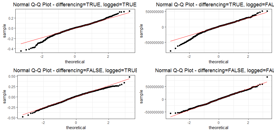
A normal distribution assumption is required for the test of the coefficients of the model. The pictures below will help you to make a decision.
do.call(grid.arrange, comparison$qqPlot)
do.call(grid.arrange, comparison$histPlot)

The following table shows the results of various models when other options have been changed, with the exception of log and differencing transformations.
At this time, up to 10 models are compared considering various combinations of options.
comparison$params
differencing logged smooth.origin synergy.promotion trend period structural.change       AIC      RMSE        MAE  p
1          TRUE   TRUE           tag             FALSE  TRUE   NULL             FALSE -1488.699 0.1101252 0.08259737  8
2          TRUE   TRUE           tag              TRUE FALSE   auto             FALSE -1492.414 0.1087691 0.08221139 18
3          TRUE   TRUE           tag             FALSE FALSE   auto             FALSE -1493.125 0.1098708 0.08260071  8 *final*
4          TRUE   TRUE           tag             FALSE FALSE   NULL             FALSE -1490.699 0.1101252 0.08259681  7
5          TRUE   TRUE           tag              TRUE FALSE   NULL              TRUE -1483.025 0.1089619 0.08221421 21
6          TRUE   TRUE           tag              TRUE  TRUE   auto              TRUE -1485.006 0.1087355 0.08218397 22
7          TRUE   TRUE           tag             FALSE FALSE   auto              TRUE -1485.148 0.1098695 0.08261233 12
8          TRUE   TRUE           tag              TRUE FALSE   NULL             FALSE -1491.008 0.1089629 0.08219880 17
9          TRUE   TRUE           tag             FALSE  TRUE   NULL              TRUE -1480.721 0.1101239 0.08260761 12
10         TRUE   TRUE           tag              TRUE  TRUE   NULL             FALSE -1489.008 0.1089628 0.08219762 18
In addition, the promotionImpact object for each model is stored in "models" in the form of a list, and the final model which minimizes AIC can be called from "final_model".