Experiments with Adversarial Autoencoders in Keras

The experiments are done within Jupyter notebooks. The notebooks are pieces of Python code with markdown texts as commentary. All remarks are welcome.

Variational Autoencoder

The variational autoencoder is obtained from a Keras blog post. There have been a few adaptations.

• There is confusion between log_sigma and log_variance. The sampling function expected standard deviation as input, but got variance as input. The variable name has been adjusted from log_sigma to log_variance and the function has been adapted: K.exp(z_log_variance / 2) rather than K.exp(z_log_sigma).
• The loss has been adjusted so that the loss is a larger number. The variable xent_loss is multiplied with original_dim and for the kl_loss, rather than K.mean, we use K.sum. The ratio between xent_loss and kl_loss is not changed.

The Python code in this other Keras github example has been used to figure out what is going on.

The results are often presented in the following manners. First, a visual inspection of the reconstruction of a familiar dataset, most often MNIST digits. Second, the test samples are encoded into the latent variable representation. The latent variables are then presented in a 2D scatterplot. Third, there is a sweep over the latent variable values to generate digits. The second and third presentations are especially useful if the encoder has only two latent variables. Then the presentation in a 2D scatterplot does not require any dimension reduction. The sweep over only two latent variables is also very easy to represent in 2D.

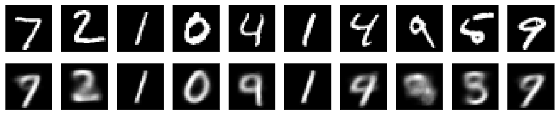
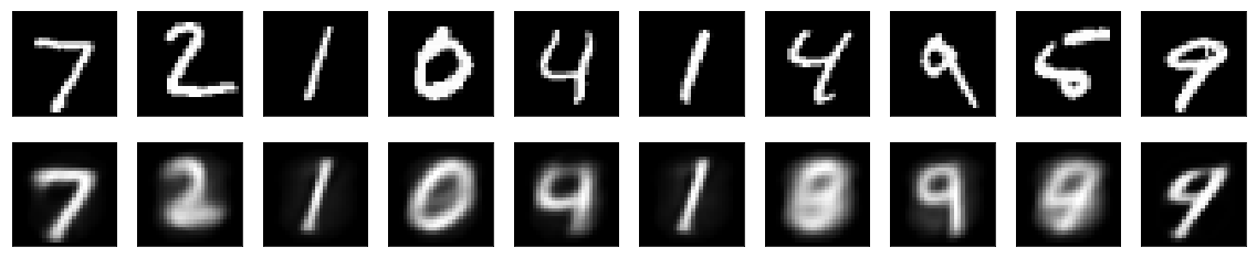
The MNIST digits are reconstructed like this by a variational autoencoder:

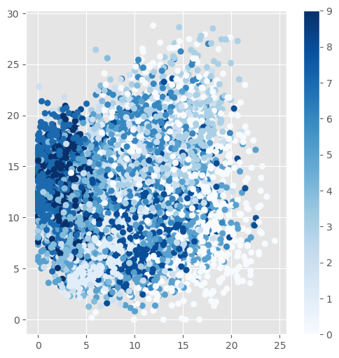
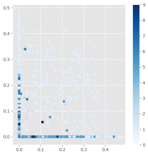
The scatterplot of the latent variable representation of the test set. It can be seen that similar digits are mapped to similar values in the latent space.

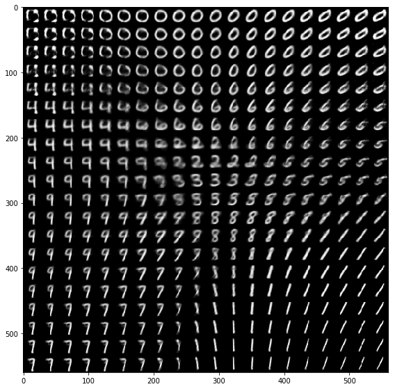
Sweeping uniformly over the two latent variables in small increments shows how it generates shapes that really look like digits. Note that not every digit is represented equally in the latent layer. Especially the zero seems to occupy a lot of the latent space. By the way, in the MNIST training set all digits are more or less uniformly distributed:

5923 0
6742 1
5958 2
6131 3
5842 4
5421 5
5918 6
6265 7
5851 8
5949 9

This is henceforth not an artifact of seeing zero more often in the dataset.

Now I'm thinking of this... Thinking out loud... It might be interesting to somehow get a grip on the "amount of space" is occupied by each digit. Assume there is a competitive structure involved. Suppose an input leads to a vastly different representation. (It is a different digit!) Now we "carve out" some repelling area around it in the latent space (by that competitive mechanism). This would mean that any sufficiently different structure would get equal say in the latent space. The only exception would be completely different manners of writing of the same digit. There is a problem with this however. It would also mean that there will be more space dedicated to (unrealistic) transitions between digits. That would be a waste of latent space.

Ordinary Autoencoder

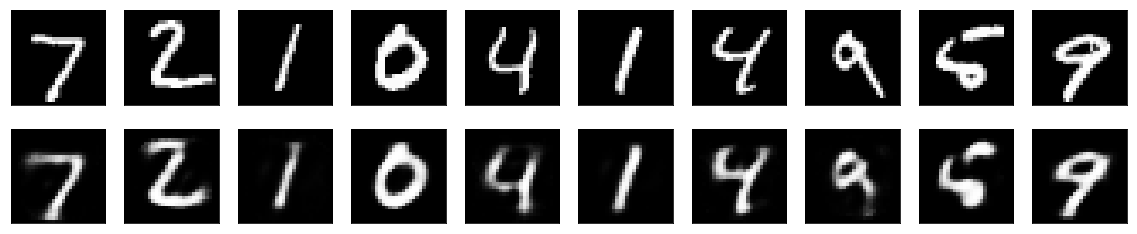
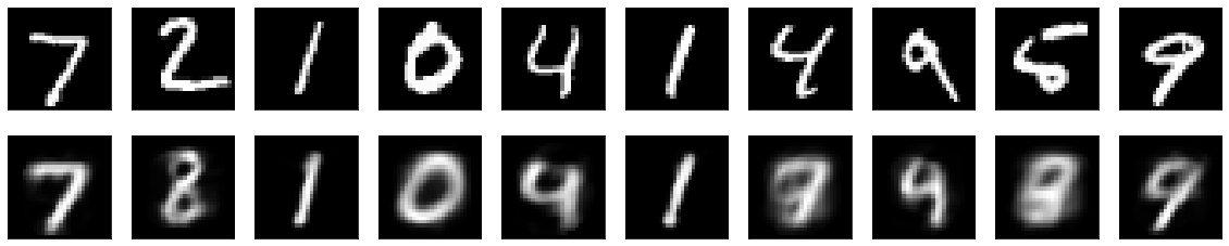
An "ordinary" autoencoder has been trained with a latent variable layer of 32 nodes (rather than 2 as in the variational autoencoder above). The reconstruction is similar to that of the variational autoencoder (using visual inspection):

The quality of the latent representation is harder to check using a scatterplot. For example, if we just use the test samples to see how they influence the first two latent variable nodes, there is not much structure to observe:

We might perform dimensionality reduction and for example use t-SNE to map to a 2D space. However, this is much more indirect than in the case that there are only two latent variables. If there is still not structure observed, it might be just an artifact of how t-SNE performs dimensionality reduction (not indicating the quality of the latent variable representation).

Sparse Autoencoder

A sparse autoencoder is similar to the ordinary autoencoder, but enforces sparsity through an "activity regularizer". On the Keras blog there is an example of a L1 regularizer. In the paper "Deep Learning of Part-based Representation of Data Using Sparse Autoencoders with Nonnegativity Constraints" by Hosseini-Asl et al. this is done by minimizing the KL divergence between the average activity of hidden units and a predefined parameter, p (both assumed to be Bernoulli random variables). The final cost function is than a weighted sum of the reconstruction error and the KL divergence. This is normally weighted through a Lagrange multiplier, beta, multiplied by the KL divergence terms.

• For MNIST digits, an L1 regularizer is used with lambda = 10e-8. If I choose 10e-5 the results are blurry. Regretfully with a KL divergence using common parameters from the literature (like p = 0.1 and beta = 3) or as mentioned in the above paper (p = 0.05 and beta = 3) I also get blurry reconstructions.
• If I use the mean in the KL term rather than the sum, it also leads to sharper images again (however, in the Sparse Autoencoder tutorial by Ng - which everybody seems to be implementing - it is actually a sum).
• When using the mean the result is actually sparse: encoded_imgs.mean() is only 0.012 (using Adam and MSE and p = 0.01, beta = 6). There is still some stuff to figure out here...
• Beta somehow seems to work if it has smaller values than the ones mentioned in the literature. With beta = 0.01 or similar values everything works out. With large values for beta the sparsity constraint takes over in such a way that the reconstruction suffers.
• Ah! Introducing a weight decay factor solves this! With p = 0.05 and beta = 3 and with a kernel_regularizer equal to regularizers.l2(0.003) we get sharper images again.

The scatterplot:

Nice to see that for most digits at least one of the first two nodes in the latent layer are indeed zero.

Nonnegative Autoencoder

An adaptation to the Sparse Autoencoder with a nonnegative constraint rather than a weight decay term can be found in this notebook.

Installation

You need to install Tensorflow, Keras, Python, SciPy/NumPy, Jupyter. Use e.g. pip3 to make installation a little bit less of a pain (but still).

sudo -H pip3 install tensorflow
sudo -H pip3 install keras
sudo -H pip3 install --upgrade --force-reinstall scipy
sudo -H pip3 install jupyter

Check your installation by running python3 and try importing it:

python3
import tensorflow as tf
import keras.backend as K

Check pip3 if you actually installed it in the "right way":

sudo -H pip3 list | grep -i keras

Copyright

• Author: Anne van Rossum
• Copyright: Anne van Rossum
• Date: July 12, 2018
• License: LGPLv3+, Apache Licensen 2.0, and/or MIT (triple-licensed)