The notes are prepared by Samrat Mitra

Deep learning (also known as deep structured learning) is part of a broader family of machine learning methods based on artificial neural networks with representation learning. Learning can be supervised, semi-supervised or unsupervised.
Deep-learning architectures such as deep neural networks, deep belief networks, deep reinforcement learning, recurrent neural networks and convolutional neural networks have been applied to fields including computer vision, speech recognition, natural language processing, machine translation, bioinformatics, drug design, medical image analysis, material inspection and board game programs, where they have produced results comparable to and in some cases surpassing human expert performance.
Artificial neural networks (ANNs) were inspired by information processing and distributed communication nodes in biological systems. ANNs have various differences from biological brains. Specifically, artificial neural networks tend to be static and symbolic, while the biological brain of most living organisms is dynamic (plastic) and analogue.
The adjective "deep" in deep learning refers to the use of multiple layers in the network. Early work showed that a linear perceptron cannot be a universal classifier, but that a network with a nonpolynomial activation function with one hidden layer of unbounded width can. Deep learning is a modern variation which is concerned with an unbounded number of layers of bounded size, which permits practical application and optimized implementation, while retaining theoretical universality under mild conditions. In deep learning the layers are also permitted to be heterogeneous and to deviate widely from biologically informed connectionist models, for the sake of efficiency, trainability and understandability, whence the "structured" part.
1. Artificial Neural Network (ANN) ✅ Google Colab File Available here

ANN Article Click Here!!
Artificial neural networks (ANNs) or connectionist systems are computing systems inspired by the biological neural networks that constitute animal brains. Such systems learn (progressively improve their ability) to do tasks by considering examples, generally without task-specific programming. For example, in image recognition, they might learn to identify images that contain cats by analyzing example images that have been manually labeled as "cat" or "no cat" and using the analytic results to identify cats in other images. They have found most use in applications difficult to express with a traditional computer algorithm using rule-based programming.
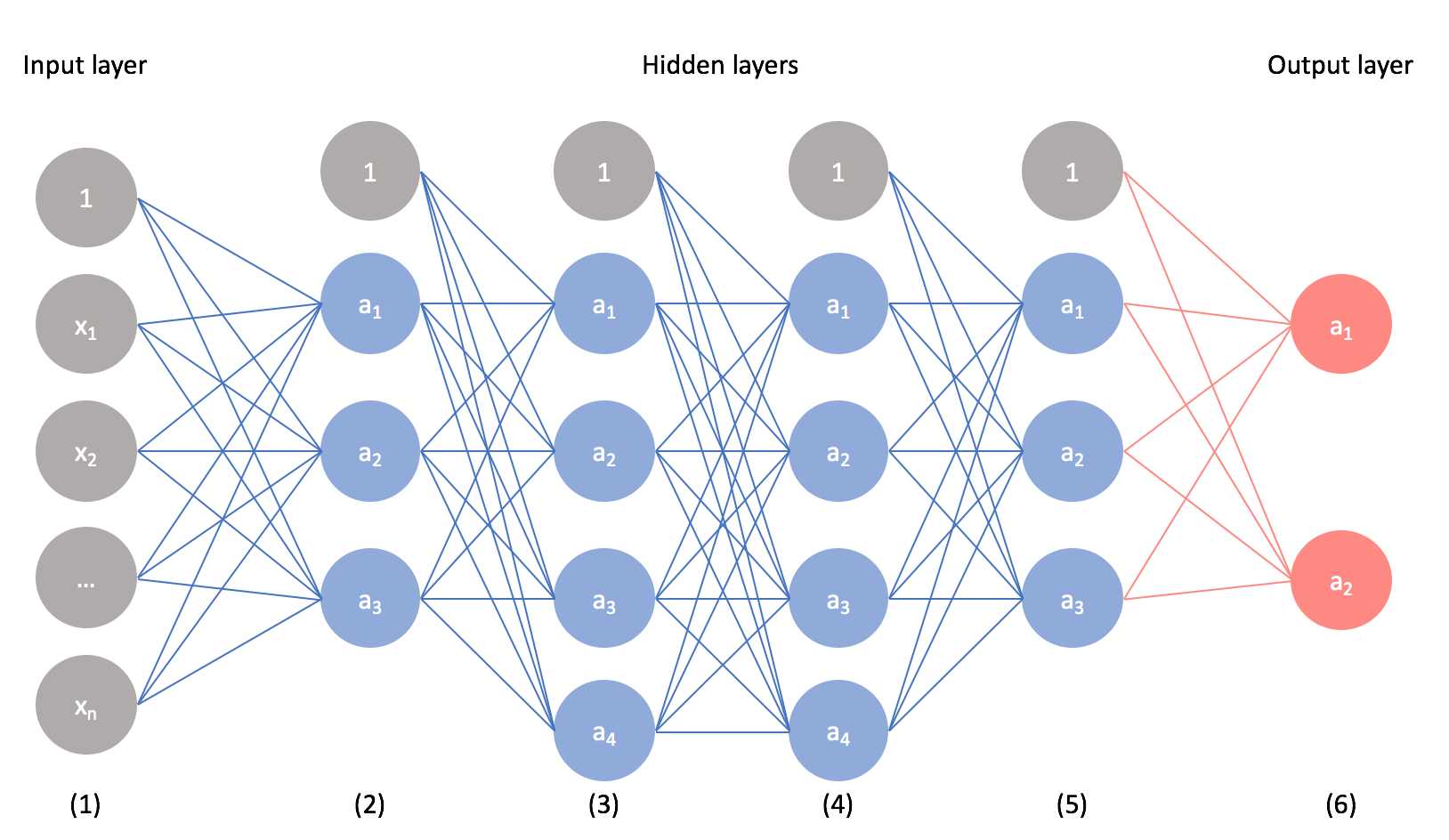
An ANN is based on a collection of connected units called artificial neurons, (analogous to biological neurons in a biological brain). Each connection (synapse) between neurons can transmit a signal to another neuron. The receiving (postsynaptic) neuron can process the signal(s) and then signal downstream neurons connected to it. Neurons may have state, generally represented by real numbers, typically between 0 and 1. Neurons and synapses may also have a weight that varies as learning proceeds, which can increase or decrease the strength of the signal that it sends downstream.
Typically, neurons are organized in layers. Different layers may perform different kinds of transformations on their inputs. Signals travel from the first (input), to the last (output) layer, possibly after traversing the layers multiple times.
The original goal of the neural network approach was to solve problems in the same way that a human brain would. Over time, attention focused on matching specific mental abilities, leading to deviations from biology such as backpropagation, or passing information in the reverse direction and adjusting the network to reflect that information.
Neural networks have been used on a variety of tasks, including computer vision, speech recognition, machine translation, social network filtering, playing board and video games and medical diagnosis.
As of 2017, neural networks typically have a few thousand to a few million units and millions of connections. Despite this number being several order of magnitude less than the number of neurons on a human brain, these networks can perform many tasks at a level beyond that of humans (e.g., recognizing faces, playing "Go" ).
2. Convolutional Neural Network (CNN) ✅ Google Colab File Available here
CNN Article Click Here!!
In deep learning, a convolutional neural network (CNN, or ConvNet) is a class of artificial neural network, most commonly applied to analyze visual imagery. They are also known as shift invariant or space invariant artificial neural networks (SIANN), based on the shared-weight architecture of the convolution kernels or filters that slide along input features and provide translation equivariant responses known as feature maps. Counter-intuitively, most convolutional neural networks are only equivariant, as opposed to invariant, to translation. They have applications in image and video recognition, recommender systems, image classification, image segmentation, medical image analysis, natural language processing, brain-computer interfaces, and financial time series.
CNNs are regularized versions of multilayer perceptrons. Multilayer perceptrons usually mean fully connected networks, that is, each neuron in one layer is connected to all neurons in the next layer. The "full connectivity" of these networks make them prone to overfitting data. Typical ways of regularization, or preventing overfitting, include: penalizing parameters during training (such as weight decay) or trimming connectivity (skipped connections, dropout, etc.) CNNs take a different approach towards regularization: they take advantage of the hierarchical pattern in data and assemble patterns of increasing complexity using smaller and simpler patterns embossed in their filters. Therefore, on a scale of connectivity and complexity, CNNs are on the lower extreme.
Convolutional networks were inspired by biological processes in that the connectivity pattern between neurons resembles the organization of the animal visual cortex. Individual cortical neurons respond to stimuli only in a restricted region of the visual field known as the receptive field. The receptive fields of different neurons partially overlap such that they cover the entire visual field.
CNNs use relatively little pre-processing compared to other image classification algorithms. This means that the network learns to optimize the filters (or kernels) through automated learning, whereas in traditional algorithms these filters are hand-engineered. This independence from prior knowledge and human intervention in feature extraction is a major advantage.
A convolutional neural network consists of an input layer, hidden layers and an output layer. In any feed-forward neural network, any middle layers are called hidden because their inputs and outputs are masked by the activation function and final convolution. In a convolutional neural network, the hidden layers include layers that perform convolutions. Typically this includes a layer that performs a dot product of the convolution kernel with the layer's input matrix. This product is usually the Frobenius inner product, and its activation function is commonly ReLU. As the convolution kernel slides along the input matrix for the layer, the convolution operation generates a feature map, which in turn contributes to the input of the next layer. This is followed by other layers such as pooling layers, fully connected layers, and normalization layers.
In a CNN, the input is a tensor with a shape: (number of inputs) x (input height) x (input width) x (input channels). After passing through a convolutional layer, the image becomes abstracted to a feature map, also called an activation map, with shape: (number of inputs) x (feature map height) x (feature map width) x (feature map channels).
Convolutional layers convolve the input and pass its result to the next layer. This is similar to the response of a neuron in the visual cortex to a specific stimulus. Each convolutional neuron processes data only for its receptive field. Although fully connected feedforward neural networks can be used to learn features and classify data, this architecture is generally impractical for larger inputs such as high resolution images. It would require a very high number of neurons, even in a shallow architecture, due to the large input size of images, where each pixel is a relevant input feature. For instance, a fully connected layer for a (small) image of size 100 x 100 has 10,000 weights for each neuron in the second layer. Instead, convolution reduces the number of free parameters, allowing the network to be deeper. For example, regardless of image size, using a 5 x 5 tiling region, each with the same shared weights, requires only 25 learnable parameters. Using regularized weights over fewer parameters avoids the vanishing gradients and exploding gradients problems seen during backpropagation in traditional neural networks. Furthermore, convolutional neural networks are ideal for data with a grid-like topology (such as images) as spatial relations between separate features are taken into account during convolution and/or pooling.
3. Recurrent Neural Network (RNN) ✅ Google Colab File Available here
RNN Article Click Here!!
Colah's Article for RNN (Best Explanation using LSTM) Click Here!!
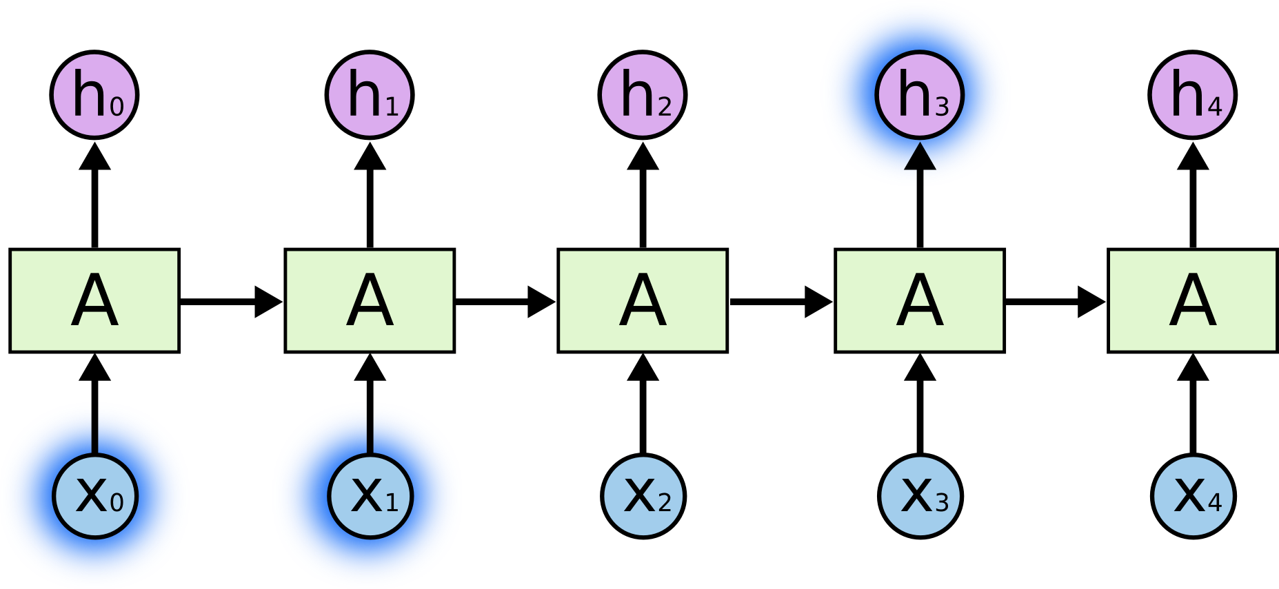
A Recurrent neural network (RNN) is a class of artificial neural networks where connections between nodes form a directed graph along a temporal sequence. This allows it to exhibit temporal dynamic behavior. Derived from feedforward neural networks, RNNs can use their internal state (memory) to process variable length sequences of inputs. This makes them applicable to tasks such as unsegmented, connected handwriting recognition or speech recognition. Recurrent neural networks are theoretically Turing complete and can run arbitrary programs to process arbitrary sequences of inputs.
The term “recurrent neural network” is used indiscriminately to refer to two broad classes of networks with a similar general structure, where one is finite impulse and the other is infinite impulse. Both classes of networks exhibit temporal dynamic behavior. A finite impulse recurrent network is a directed acyclic graph that can be unrolled and replaced with a strictly feedforward neural network, while an infinite impulse recurrent network is a directed cyclic graph that can not be unrolled.
Both finite impulse and infinite impulse recurrent networks can have additional stored states, and the storage can be under direct control by the neural network. The storage can also be replaced by another network or graph if that incorporates time delays or has feedback loops. Such controlled states are referred to as gated state or gated memory, and are part of long short-term memory networks (LSTMs) and gated recurrent units. This is also called Feedback Neural Network (FNN).
Long short-term memory (LSTM) networks were invented by Hochreiter and Schmidhuber in 1997 and set accuracy records in multiple applications domains.
Around 2007, LSTM started to revolutionize speech recognition, outperforming traditional models in certain speech applications. In 2009, a Connectionist Temporal Classification (CTC)-trained LSTM network was the first RNN to win pattern recognition contests when it won several competitions in connected handwriting recognition. In 2014, the Chinese company Baidu used CTC-trained RNNs to break the 2S09 Switchboard Hub5'00 speech recognition dataset benchmark without using any traditional speech processing methods.
LSTM also improved large-vocabulary speech recognition and text-to-speech synthesis and was used in Google Android. In 2015, Google's speech recognition reportedly experienced a dramatic performance jump of 49%[citation needed] through CTC-trained LSTM.
LSTM broke records for improved machine translation, Language Modeling and Multilingual Language Processing. LSTM combined with convolutional neural networks (CNNs) improved automatic image captioning.

RNNs come in many variants.
Fully recurrent neural networks (FRNN) connect the outputs of all neurons to the inputs of all neurons. This is the most general neural network topology because all other topologies can be represented by setting some connection weights to zero to simulate the lack of connections between those neurons. The illustration to the right may be misleading to many because practical neural network topologies are frequently organized in "layers" and the drawing gives that appearance. However, what appears to be layers are, in fact, different steps in time of the same fully recurrent neural network. The left-most item in the illustration shows the recurrent connections as the arc labeled 'v'. It is "unfolded" in time to produce the appearance of layers.
