Regression

Introduction

In this blog series, we will discuss major important topics that will form a base for Machine Learning which are

- Simple Linear Regression 
- Multiple Linear Regression
- Lasso Regression
- Ridge Regression
- Kernel Regression
- K-Nearest Neighbor

So particularly in this blog, we are gonna discuss Simple Linear Regression, Optimization algorithm, Residual Sum of Squares & how to minimize it.

What is Regression?

Regression analysis is a form of predictive modelling technique which investigates the relationship between a dependent and an independent variable.

The above definition is bookish, in simple terms the regression can be defined as, Using the relationship between variables to find the best fit line or the regression equation that can be used to make prediction.

There are many types of regressions such as Linear Regression, Polynomial Regression, Logistic regression and various other Regression algorithms but in this blog, we are gonna study Simple Linear Regression, Multiple Linear Regression, Lasso Regression, Ridge Regression, Kernel Regression & K-Nearest Neighbor Regression.

Linear Regression

Before going into deep, let's first discuss some terminology, examples related to regression so that we can understand it better later.

So suppose you want to sell your house and you want to predict the price of your house based on the size of the house then you can easily predict the price of a house using Simple Linear Regression.

So Data will be like

In the dataset above, we can see there is one input parameter which is the size of the house(square ft) while the output of our regression model will be the price of the house($$$).

Assumptions in Regression

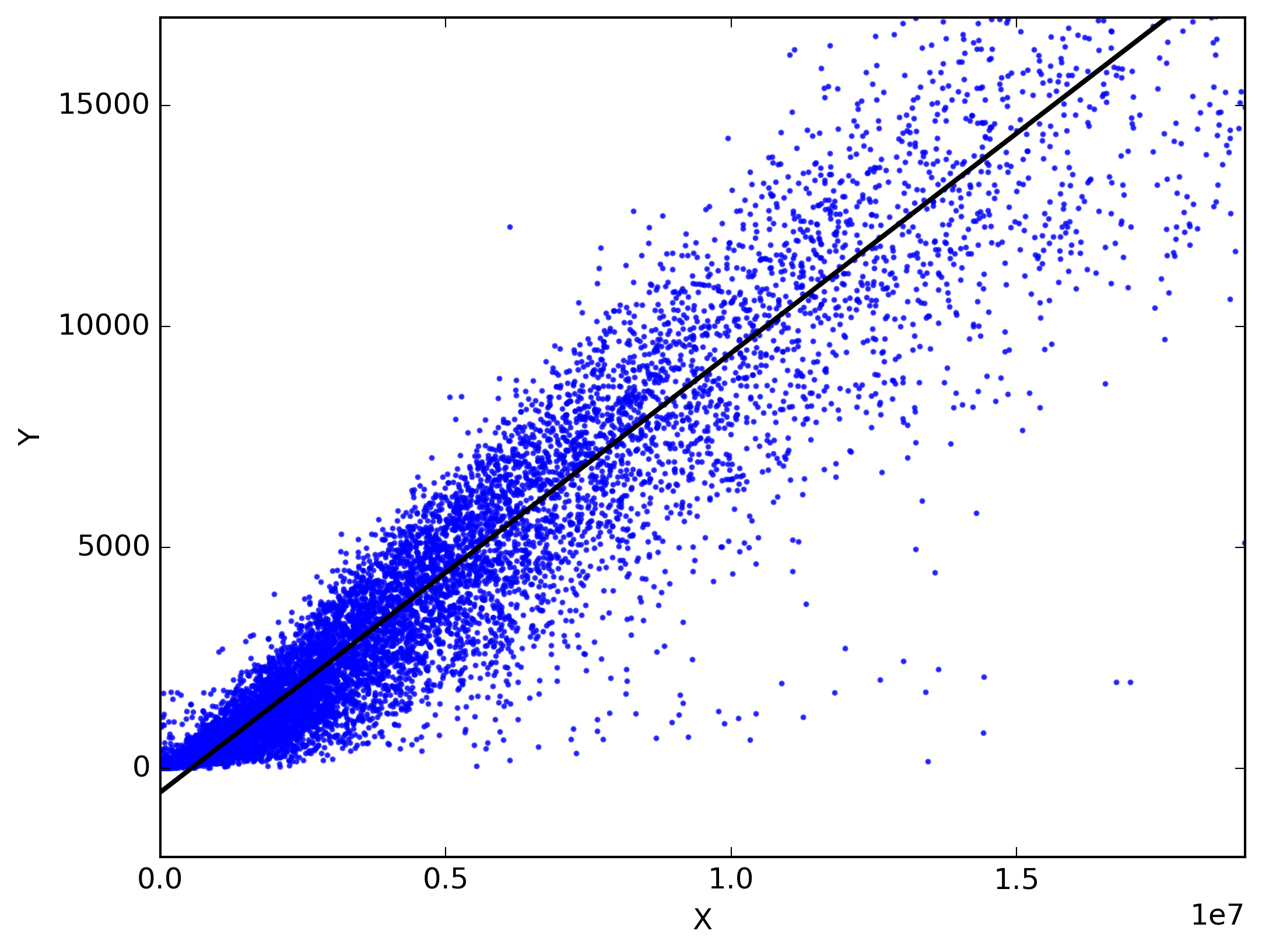
From the image above it can be seen that there are some points scatter on the 2D space where Y-axis is the price($$$) of the house and X-axis is the size(sq. ft.) of the house and points are scattered according to that. Then there is a green line which we call as the function (f(x)) best fitting on our data(we will see later).

But we can see that our function does not pass through all the data points. So if we take a point X _I marked blue in the image above we see that there is a gap between the original value and predicted the value at X _I . This gap is called as the error(ε_i).

Similarly, there is some error in all the predicted value of the data points.

We here assume that expected value of ε_i is 0 i.e.,

By this equation, we meant that it's equally likely that our error is positive or negative. And what does this imply? This implies that it's equally likely that our observation, the specific observation that we get, is above or below the functional relationship defined by f(x _I ). So, y_i is equally likely to be above or below, f(x_i).

I want to be clear that this is the model that we're using. This is how we're assuming the world works. And there's this very famous quote by George Box that says, Essentially, all models are wrong, but some are useful. So what this means is no models going to be exactly how the world works. It's not going to exactly predict how houses sell, just based on square feet, or even if you incorporated other things as well. There's always different idiosyncrasies in how the world works. So above we have discussed the assumption had been taken while designing the algorithm.

So we are now gonna discuss the life cycle of a Machine Learning algorithm.

So every machine learning algorithm start with training data which includes several features/attributes here in our example of house price prediction there can be many attributes such as house id, house sales, location of a house, number of rooms etc... then all those attributes are passed onto next where the feature selection happens i.e. it is not necessary that all the features in the dataset are good for the prediction of the house price after doing feature selection via many algorithms(we will discuss later in the blog) we have all the important features of the dataset then we will pass them through an ML model which will predict the price of a house.

So now we have the predicted price of a house but we should have some metrics system which will tell how much close we have predicted the price or how much accurate our algorithm is. After calculating the errors in the prediction we will again train our Machine Learning algorithm on the data and repeat the process again and again till we reach to the required accuracy.

So this is the life cycle of Machine Learning algorithm on every dataset.

Now we have basic knowledge regarding Machine Learning, let's explore various Regression algorithms.

Simple Linear Regression

Simple linear regression is a linear regression model with a single variable as input. That is, it concerns two-dimensional sample points with one independent variable and one dependent variable (conventionally, the x and y coordinates in a Cartesian coordinate system) and finds a linear function (a non-vertical straight line) that, as accurately as possible, predicts the dependent variable values as a function of the independent variables. It is the simplest form of all regression algorithms.

So going back to our flowchart, what we're gonna talk about now is specifically the machine learning model. So that's highlighted green box and everything else is greyed out so you can forget about everything else for now. We're just talking about our model and what form it takes. So our Simple Linear Regression model is just that. It's very simple. We're assuming we have just one input, which in this case is, square feet of the house and one output which is the house sales price and we're just gonna fit a line. A very simple function here not that quadratic function or higher-order polynomials we talked about before, just a very simple line. And what's the equation of a line?

Well, it's just intercept plus slope times our variable of interest so that we're gonna say that's W₀+ W₁x. And what this regression model then specifies is that each one of our observations y_i is simply that function evaluated at X_i. So that's W₀ plus W_i * X_i plus the error term which we called ε_i. So this is our regression model, and to be clear, this error, ε_i, is the distance from our specific observation back down to the line.

Equation of Simple Linear Regression is,

While that for any point on the 2D space is,

In the equation of Simple Linear Regression, we can see that it is nothing but an equation of Straight Line where, slope is w_i while intercept is w₀, y_i is our prediction and x_i is our input which is the size of the house. Slope and intercept here are called parameters: regression coefficients. We will explore then in details later in the blog.

Fitting line to the data

While working with a Simple Linear Regression model, let's talk about how we're gonna fit a line to data. But before we talk about specific algorithms for fitting, we need to talk about how we're gonna measure the quality of a fit. So, we're gonna talk about this orange box in the above image which is quality metric.

So here the metric we are going to use is called Residual Sum of Errors also abbreviated as RSS. It is nothing but the sum of squares of the difference between the original price of the house and predicted the price of the house by our model over the whole training dataset i.e.,

Above dangerously looking equation can be compressed as below using Sigma(Σ) notation,

Above equation can also be written as,

Where y_hat is our prediction at each data point and we calculate it's difference from the original value, then we are squaring it and doing the sum of all the squares at each data points to calculate the overall cost.

Now we have overall cost of a particular Regression model, we can try the different possible combination of parameters i.e., w₀ and w₁ which will give different cost and we will take that line which had a minimum cost.

So now the questions arise till when we keep on searching the values for parameters and how we will get to know whether the parameters we got are one having the minimum cost on our dataset i.e. best parameters for the dataset.

So to solve this problem there comes the concept of optimization algorithms which will tell us that when to stop and provide us with the best parameters for the dataset. There are several optimization techniques like Gradient Descent, Coordinate Descent, Adam, RMP prop, Momentum but we are gonna discuss only Gradient Descent and Coordinate descent in the blog.

Before discussing the optimization algorithm we will first discuss the interpretation of the parameters in the equation of the Simple Linear Regression

Use & Interpretation of the fitted Line

The above Regression model can be used by the seller as well as by the buyers both. Here it is how.

Seller can put the size of his/her house in the equation and can easily predict the house price which he/she wanted to sell.

Similarly, a buyer can put his/her budget in the equation and can know how much bigger house he/she can buy in their budget.

Interpreting the coefficients

W₀ is nothing but it's the price of the house when the size of the house is 0 which doesn't make sense but W₀ doesn't have any meaning full interpretation.

W₁ is the slope of the line which here means that it is predicted the change in the price of the house(output) per unit change in the size of the house(input).

We have seen the metrics(RSS) which we will be using to decide whether parameters of a particular model are good enough for the dataset & to decide the best model for a dataset. Let now see the algorithms for fitting the model.

Algorithm for fitting the model

Now that we have an understanding of what the fitted line is, and how we can use it, let's talk about an algorithm for searching out the space of all possible lines that we might use, and finding the one that best fits the data. So in particular what we're going to be doing is focusing in on this machine learning algorithm, which is this dark grey square is shown in the above flow chart.

So recall that our cost was to find us this Residual Sum of Squares, and for any given line, we can compute the cost of that line. So, for example, we showed three different lines and three different residual sums of squares here, but our goal was to minimize over all possible W0 and W1 slopes and intercepts, but a question is, how are we going to do this? So that's the key question that we're looking to address in this section.

Let's formalize this idea a little bit more. So here, what we're showing is our Residual Sum of Squares and what we see is it's a function of two variables, w₀ and w₁. So we can write it generically, let's just write it as some function g of a variable w₀ and a variable w₁. And what I've done is I've gone ahead and plotted the residual sum of squares versus w₀ and w₁ for the data set.

So here along X-axis is w₀ and along Y-axis is w₁. And then we are plotting here our Residual Sum of Squares. And the blue mesh surface in the image is our Residual Sum of Squares for any given w₀, w₁ pair. And our objective here is to minimize over all possible combinations of w₀, and w₁.

So we want to find the specific value of w₀. So, we'll call that w₀ hat & w₁ hat, that minimize this Residual Sum of Squares. So, this is our objective. This is an optimization problem, where specifically the optimization objective is to minimize a function, in this case, of two parameters, two different variables

So now we are gonna discuss some optimization techniques which will give us the best parameters, w₀ hat & w₁ hat which minimizes the Residual Sum of Squares thereby providing us with the best model, but before that we have to discuss some terminologies like what is Concavity, Convexity and other related terms.

An aside on Optimization

Concave/Convex functions

Given a function g(w) if we construct a line starting at point (a, g(a)) and ending at point (b, g(b)) then the line always lie below the function g(w) then this type of functions are known as Concave functions.

And if, given a function g(w) if we construct a line starting at point (a, g(a)) and ending at point (b, g(b)) then if line always lie above the function g(w) then this type of functions are known as Convex functions.

Last but not the least, given a function g(w) if we construct a line starting at point (a, g(a)) and ending at point (b, g(b)) then if line sometimes lie above the function & sometimes lie below the function then this type of functions are neither Convex nor Concave.

Below are examples of each case.

Now we know what is Concavity and Convexity, let's discuss how to find maximum and minimum of a function because our cost which is Residual Sum of Squares is Convex and we have to find the parameters that minimize our cost on the dataset.

In case of Concave function we can only find maximum value while in case of Convex functions we can only find a minimum value.

To find the minimum and maximum values in Convex and Concave functions respectively we have to take the first derivative of the function and make the derivative of the function as zero and calculate the value where that derivative is zero. The value where a derivative is zero will give the minimum and maximum value in Convex and Concave respectively.

In case of neither Concave nor Convex function there can be multiple maximum and minimum values.

Let's look at the example below.

Finding Maximum via Hill Climbing

We can find maximum/minimum by setting the first derivative to zero but there are many functions which are non-derivable i.e., we can't take their derivative so in that case we are gonna use this Hill Climbing/Descent algorithm.

So in this algorithm, we start from a point and we aim to reach to the value where the function takes the maximum value. But we don't know whether we have to move forward or backwards to reach to maximum value???

So at each iteration, we will take the derivative of the function and check whether it is positive or negative. If it is negative then we have to move backwards while if it's positive then we have to move forward (as it is Concave function).

So algorithm is,

Finding Minimum via Hill Descent

We can find maximum/minimum by setting the first derivative to zero but there are many functions which are non-derivable i.e., we can't take their derivative so in that case we are gonna use this Hill Climbing/Descent algorithm.

So in this algorithm, we start from a point and we aim to reach to the value where the function takes the minimum value. But we don't know whether we have to move forward or backwards to reach to minimum value???

So at each iteration, we will take the derivative of the function and check whether it is positive or negative. If it is negative then we have to move forward while if it's positive then we have to move backwards (as it is Convex function).

So algorithm is,

So now we know how to find the maximum/minimum value of a function but there are few sceptical things in the algorithm which you will be thinking how to decide them. So now we are gonna discuss how to decide them i.e., we will explore what η the value we should take and what should be the convergence criteria for algorithm i.e., when we have to stop the algorithm.

Choosing the Stepsize(η)

Stepsize(η) decides how much time it will take to the algorithm to reach to minimum/maximum value of the function. If η is very high then there are chances that we may overshoot the required parameters and will never reach to that value again and if η value is very small then it will take a long time for the algorithm to find the required parameters. So it's kind of art to find the optimum value of stepsize for the dataset.

It is suggested to take Stepsize where initially it's values is relatively large, as our algorithm progresses it's value keeps on decreasing because initially, we start from a random value of parameters so we want to take big steps to converge fast but after each iteration, we are more close to optimum parameters so after some iterations, we are more close to required parameters so we don't want to overshoot them, therefore, we take the step size in such a way that initially, it is large and keeps on decreasing after each iteration.

Some common choices for Stepsize are,

If we take the fixed Stepsize then we may reach to the optimum parameters but the motion will be like,

Convergence criteria

For Convex functions we can find the optimum value when the first derivative is set to zero but in practice, where there may be chances that the function may not be derivable so we never use this method i.e., finding the first derivative and setting it to zero. We always use Hill Climbing/Descent algorithm and in Machine Learning we always want to minimize the cost and our cost functions are also Convex for we are gonna use Hill Descent algorithm.

In practice we will stop the algorithm when the magnitude of the First Derivative is less than some threshold(ε) set by us only. The reason for this is that in practice, we can never get to the minimum of the function because of randomness in the dataset so we are happy with the parameters that are exactly not optimum but very near to the optimum parameters.

But as we know that input attributes are not a single(except Simple Linear Regression) attribute so instead of taking the derivative we will take partial derivative w.r.t every attribute of the dataset and we will call it as Gradient of the function and our algorithm's name Hill Descent is changed to Gradient Descent in multiple dimensions.

Gradient Example

Gradient Descent algorithm

It is similar to Hill Descent algorithm. It is an iterative algorithm which stops only when the magnitude of the Gradient is less than the specified threshold (ε). The only difference between Hill Descent & Gradient Descent is that instead of calculating the First Derivative we will be calculating the Gradient because here there is multi- dimensional input instead of a single feature as input.

Convergence Criteria

Contour plot

It is nothing but a way of visualising the Gradient Descent algorithm in 2D. It's actually Bird's Eye View of the algorithm.

Finding the best line

So now we know about optimization so we can think about applying optimization algorithms that we described to our specific scenario of interest. Which is searching over all possible lines and finding the line that best fits our data.

The first thing that's important to mention is the fact that our objective is Convex. So we can go and show that this is a Convex function. And what this implies is that the solution to this minimization problem is unique. We know there's a unique minimum to this function. And likewise, we know that our Gradient Descent algorithm will converge to this minimum.

It sounds like a very complicated problem that we have to search over all possible lines to find the best fitting line to our dataset. And, of course, we couldn't possibly go and test each one of these lines, so we can use the very straightforward optimization algorithms that we described above and solve for the solution to the problem.

Let's return to the definition of our cost, which is the Residual Sum of Squares of our two parameters, (w₀, w₁). To find the optimum parameters through Gradient Descent we have to compute the Gradient.

Our Residual Sum of Squares is,

Computing Gradient of the RSS w.r.t W₀

Computing Gradient of the RSS w.r.t W₁

Putting it all together

Well we have the Gradients so we can apply two approaches to get the optimum parameters

Approach 1

We can take the Gradient and set it equal to zero. After applying this approach to the Gradients we get the following values for our parameters

Above parameters can be simplified to the following,

W₀ = (mean of Y) - slope * (mean of X) W₁ = ((mean of X * Y) - (mean of X)(mean of Y))/ ((mean of X^2) - (mean of X)(mean of X))

Approach 2

Instead of setting Gradient to zero we can apply Gradient Descent algorithm

Let's interpret the parameters W₀ & W₁ obtained from the Gradient Descent.

From the above image we can see that in W₀ a term is added which is nothing but the difference between the original price of the house and predicted price of the house. So if suppose we are always under predicting the price of the house then y_i - y_hat_i is going to be positive then we are increasing the weights. In other words, since we are under predicting the price which means that our predicted line is lower than it should be so we are pushing it in upward direction thereby, trying to fit the data as much good as possible.

Similar intuition for W₁, just here we are adding (y_i - y_hat_i) * X_i

Comparing two Approaches

We've gone over, either setting the gradient equal to zero or doing gradient descent. Well, in the case of minimizing Residual Sum of Squares, we showed that both were fairly straight forward to do. But in a lot of the machine learning method's that we're interested in taking the gradient and setting it equal to zero, well there's just no closed-form solution in many cases.

So, often we have to turn to method's like Gradient Descent. And likewise, we are gonna see in next blogs that where we turn to have lots of different inputs, lots of different features in our Regression, even though there might be a closed-form solution to setting the gradient equal to zero, sometimes in practice, it can be much more efficient computationally to implement the Gradient Descent approach.

And finally one thing that I should mention about the Gradient Descent approach is the fact that in that case, we had to choose a step size and a convergence criteria which, of course, is a downside to the Gradient Descent approach, is having to specify these parameters of the algorithm. But many times we're relying on these types of Optimization algorithms to solve our problems.

Conclusion & Sumary for Simple Linear Regression

So in this blog I've talked about Simple Linear Regression. And what we've seen is we've described what the model is. We just have a single input, single output, and fitting a line or model. It's just a simple line, to describe the relationship between our input X and our output y.

We've talked about goodness of fit of a specific line to our data and the measure being the Residual Sum of Squares. We've also talked about some ways to think about interpreting our fitted line and using it to form predictions.

But a big emphasis was on thinking about how do we actually fit that line to the data, and we talked about different Optimization techniques. The big one being, Gradient Descent, and using that to minimize our Residual Sum Squares, to come up with our fitted line that we're gonna use for predictions. Even though this is a very very simple and basic tool, it's actually incredibly powerful.

In the next blog of this series we will go through concepts of Multiple Linear Regression model in detail.

What all you can do now

References

Machine Learning Specialization Course 2 from University of Washington.

If you liked the blog, follow my GitHub(@kampaitees) to get updates about the upcoming articles. Also, share this article so that it can reach out to the readers who can gain knowledge from this. Please feel free to discuss anything regarding the post. I would love to hear feedback from you guys.