Uncertainty-Informed Deep Learning Models Enable High-Confidence Predictions for Digital Histopathology
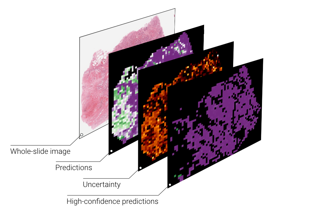
What does BISCUIT do? Bayesian Inference of Slide-level Confidence via Uncertainty Index Thresholding (BISCUIT) is a uncertainty quantification and thresholding schema used to separate deep learning classification predictions on whole-slide images (WSIs) into low- and high-confidence. Uncertainty is estimated through dropout, which approximates sampling of the Bayesian posterior, and thresholds are determined on training data to mitigate data leakage during testing.
- Python >= 3.7
- Tensorflow >= 2.7.0 (and associated pre-requisites)
- Slideflow >= 1.1.0 (and associated pre-requisites)
- Whole-slide images for training and validation
Please refer to our Installation instructions for a guide to installing Slideflow and its prerequisites.
The final uncertainty-enabled model, trained on the full TCGA dataset to predict lung adenocarcinoma vs. squamous cell carcinoma, is available on Hugging Face.
This README contains instructions for the following:
The first step to reproducing results described in our manuscript is downloading whole-slide images (*.svs files) from The Cancer Genome Atlas (TCGA) data portal, projects TCGA-LUAD and TCGA-LUSC, and slides from the Clinical Proteomics Tumor Analysis Consortium (CPTAC) data portal, projects CPTAC-LUAD and CPTAC-LSCC.
We use Slideflow for deep learning model training, which organizes data and annotations into Projects. The provided configure.py script automatically sets up the TCGA training and CPTAC evaluation projects, using specified paths to the training slides (TCGA) and evaluation slides (CPTAC). This step will also segment the whole-slide images into individual tiles, storing them as *.tfrecords for later use.
python3 configure.py --train_slides=/path/to/TCGA --val_slides=/path/to/CPTAC
Pathologist-annotated regions of interest (ROI) can optionally be used for the training dataset, as described in the Slideflow documentation. To use ROIs, specify the path to the ROI CSV files with the --roi argument.
The next step is training the class-conditional GAN (StyleGAN2) used for generating GAN-Intermediate images. Clone the StyleGAN2-slideflow repository, which has been modified to interface with the *.tfrecords storage format Slideflow uses. The GAN will be trained on 512 x 512 pixels images at 400 x 400 micron magnification. Synthetic images will be resized down to the target project size of 299 x 299 pixels and 302 x 302 microns during generation.
Use the train.py script in the StyleGAN2 repository to train the GAN. Pass the gan_config.json file that the configure.py script generated earlier to the --slideflow flag.
python3 train.py --outdir=/path/ --slideflow=/path/to/gan_cofig.json --mirror=1 --cond=1 --augpipe=bgcfnc --metrics=none
To create GAN-Intermediate images with latent space embedding interpolation, use the generate_tfrecords.py script in the StyleGAN2-slideflow repository. Flags that will be relevant include:
--network: Path to network PKL file (saved GAN model)--tiles: Number of tiles per tfrecord to generate (manuscript uses 1000)--tfrecords: Number of tfrecords to generate--embed: Generate intermediate images with class embedding interpolation.--name: Name format for tfrecords.--class: Class index, if not using embedding interpolation.--outdir: Directory in which to save tfrecords.
For example, to create tfrecords containing synthetic images of class 0 (LUAD / adenocarcinoma):
python3 generate_tfrecords.py --network=/path/network.pkl --tiles=1000 --tfrecords=10 --name=gan_luad --class=0 --outdir=gan/
To create embedding-interpolated intermediate images:
python3 generate_tfrecords.py --network=/path/network.pkl --tiles=1000 --tfrecords=10 --name=gan --embed=1 --outdir=gan/
Subsequent steps will assume that the GAN tfrecords are in the folder gan/.
Next, models are trained with train.py. Experiments are organized by dataset size, each with a corresponding label. The experimental labels for this project are:
| ID | n_slides |
|---|---|
| AA | full |
| U | 800 |
| T | 700 |
| S | 600 |
| R | 500 |
| A | 400 |
| L | 350 |
| M | 300 |
| N | 250 |
| D | 200 |
| O | 176 |
| P | 150 |
| Q | 126 |
| G | 100 |
| V | 90 |
| W | 80 |
| X | 70 |
| Y | 60 |
| Z | 50 |
| ZA | 40 |
| ZB | 30 |
| ZC | 20 |
| ZD | 10 |
Experiments are performed in 6 steps for each dataset size:
- Train cross-validation (CV) models for up to 10 epochs.
- Train CV models at the optimal epoch (1).
- Train UQ models in CV, saving predictions and uncertainty.
- Train nested-UQ models, saving predictions, for uncertainty threshold determination.
- Train models at the full dataset size without validation.
- Perform external evaluation of fully-trained models.
We perform three types of experiments:
reg: Regular experiments with balanced outcomes (LUAD:LUSC).ratio: Experiments testing varying degrees of class imbalance.gan: Cross-validation experiments using varying degrees of GAN slides in training/validation sets.
Specify which category of experiment should be run by setting its flag to True. Specify the steps to run using the --steps flag. For example, to run steps 2-6 for the ratio experiments, do:
python3 train.py --steps=2-6 --ratio=True
Once all models have finished training (the published experiment included results from approximately 1000 models, so this may take a while), results can be viewed with the results.py script. The same experimental category flags, --reg, --ratio, and --gan, are used to determine which results should be viewed. There are two additional categories of results that can be displayed:
--heatmap: Generate the heatmap shown in Figure 4.--umaps: Generates UMAPs shown in Figure 5.
Figures and output will then be saved in the results/ folder. For example:
python3 results.py --ratio=True --umaps=True
You can also use BISCUIT to supervise custom experiments, including training, evaluation, and UQ thresholding.
Start by creating a new project, following the Project Setup instructions in the Slideflow documentation. Briefly, projects are initialized by creating an instance of the slideflow.Project class and require a pre-configured set of patient-level annotations in CSV format:
import slideflow as sf

project = sf.Project(
    '/project/path',
    annotations='/patient/annotations.csv'
)
Once the project is configured, add a new dataset source with paths to whole-slide images, optional tumor Regions of Interest (ROI) files, and destination paths for extracted tiles/tfrecords:
project.add_source(
    name="TCGA_LUNG",
    slides="/path/to/slides",
    roi="/path/to/ROI",
    tiles="/tiles/destination",
    tfrecords="/tfrecords/destination"
)
This step should automatically attempt to associate slide names with the patient identifiers in your annotations CSV file. After this step, double check that your annotations file has a "slide" column for each annotation entry corresponding to the filename (without extension) of the corresponding slide. You should also ensure that the outcome labels you will be training to are correctly represented in this file.
The next step is to extract tiles from whole-slide images, using the sf.Project.extract_tiles() function. This will save image tiles in the binary *.tfrecord format in the destination folder you previously configured.
project.extract_tiles(
    tile_px=299,  # Tile size in pixels
    tile_um=302   # Tile size in microns
)
A PDF report summarizing the tile extraction phase will be saved in the TFRecords directory.
Next, set up a BISCUIT Experiment, configuring your class labels and training project.
from biscuit import Experiment

experiment = Experiment(
    train_project=project, # Slideflow training project
    outcome="some_header", # Annotations header with labels
    outcome1="class1",     # First class
    outcome2="class2"      # Second class
)
Next, train models in cross-validation using uncertainty quantification (UQ), which estimates uncertainty via dropout. Model hyperparameters can be manually configured with sf.model.ModelParams. Alternatively, the hyperparameters we used in the above manuscript can be accessed via biscuit.hp.nature2022. The uq parameter should be set to True to enable UQ.
import biscuit

# Set the hyperparameters
hp = biscuit.hp.nature2022
hp.uq = True

# Train in cross-validation
experiment.train(
    hp=hp,                  # Hyperparameters
    label="EXPERIMENT"      # Experiment label/ID
    save_predictions='csv'  # Save predictions in CSV format
)After the outer cross-validation models have been trained, the inner cross-validation models are trained so that optimal UQ thresholds can be found. Initialize the nested cross-validation training with the following:
experiment.train_nested_cv(hp=hp, label="EXPERIMENT")The experimental results for each cross-fold can either be manually viewed by opening results_log.csv in each model directory, or with the following functions:
cv_models = biscuit.find_cv(
    project=project,
    label="EXPERIMENT",
    outcome="some_header"
)
# Print patient-level AUROC for each model
for m in cv_models:
    results = biscuit.get_model_results(
        m,
        outcome="some_header",
        epoch=1
print(m, results['pt_auc'])Finally, UQ thresholds are determined from the previously trained nested cross-validation models. Use Experiment.thresholds_from_nested_cv() to calculate optimal thresholds, and then apply these thresholds to the outer cross-validation data, rendering high-confidence predictions.
df, thresh = experiment.thresholds_from_nested_cv(
    label="EXPERIMENT"
)
thresh will be a dictionary of tile- and slide-level UQ thresholds, and the slide-level prediction threshold. df is a pandas DataFrame containing the thresholded, high-confidence UQ predictions from outer cross-validation.
>>> print(df)
     id  n_slides  fold       uq  patient_auc  patient_uq_perc  slide_auc  slide_uq_perc
0  TEST     359.0   1.0  include     0.974119         0.909091   0.974119       0.909091
1  TEST     359.0   2.0  include     0.972060         0.840336   0.972060       0.840336
2  TEST     359.0   3.0  include     0.901786         0.873950   0.901786       0.873950
>>> print(thresh)
{'tile_uq': 0.008116906, 'slide_uq': 0.0023400568179163194, 'slide_pred': 0.17693227693333335}Plots can be generated showing the relationship between predictions and uncertainty, as shown in Figure 3 of the manuscript. The biscuit.plot_uq_calibration() function will generate these plots, which can then be shown using plt.show():
import matplotlib.pyplot as plt

experiment.plot_uq_calibration(
    label="EXPERIMENT",
    **thresh  # Pass the thresholds from the prior step
)
plt.show()
For reference, the full script to accomplish the above custom UQ experiment would look like:
import matplotlib.pyplot as plt
import slideflow as sf
import biscuit
from biscuit import Experiment

# Set up a project
project = sf.Project(
    '/project/path',
    annotations='/patient/annotations.csv'
)
project.add_source(
    name="TCGA_LUNG",
    slides="/path/to/slides",
    roi="/path/to/ROI",
    tiles="/tiles/destination",
    tfrecords="/tfrecords/destination"
)

# Extract tiles from slides into TFRecords
project.extract_tiles(
    tile_px=299,  # Tile size in pixels
    tile_um=302   # Tile size in microns
)

# Set up the experiment
experiment = Experiment(
    train_project=project, # Slideflow training project
    outcome="some_header", # Annotations header with labels
    outcome1="class1",     # First class
    outcome2="class2"      # Second class
)

# Train cross-validation (CV) UQ models
hp = biscuit.hp.nature2022
hp.uq = True
experiment.train(
    hp=hp,                  # Hyperparameters
    label="EXPERIMENT"      # Experiment label/ID
    save_predictions='csv'  # Save predictions in CSV format
)

# Train the nested CV models (for thresholds)
experiment.train_nested_cv(hp=hp, label="EXPERIMENT")

# Show the non-thresholded model results
cv_models = biscuit.find_cv(
    project=project,
    label="EXPERIMENT",
    outcome="some_header"
)
for m in cv_models:
    results = biscuit.get_model_results(
        m,
        outcome="some_header",
        epoch=1)
    print(m, results['pt_auc'])  # Prints patient-level AUC for each model

# Calculate thresholds from the nested CV models
df, thresh = experiment.thresholds_from_nested_cv(
    label="EXPERIMENT"
)

# Plot predictions vs. uncertainty
experiment.plot_uq_calibration(
    label="EXPERIMENT",
    **thresh  # Pass the thresholds from the prior step
)
plt.show()Alternatively, you can use the uncertainty thresholding algorithm directly on existing data, outside the context of a Slideflow project (e.g. data generated with another framework). You will need tile-level predictions from a collection of models, such as from nested cross-validation, to calculate the thresholds. The thresholds are then applied to a set of tile-level predictions from a different model. Organize predictions from each model into separate DataFrames, each with the columns:
- y_pred: Tile-level predictions.
- y_true: Tile-level ground-truth labels.
- uncertainty: Tile-level uncertainty.
- slide: Slide labels.
- patient: Patient labels (optional).
>>> dfs = [pd.DataFrame(...), ...]
>>> target_df = pd.DataFrame(...)
Calculate UQ thresholds from your cross-validation predictions with biscuit.threshold.from_cv(). This will return a dictionary with tile- and slide-level UQ and prediction thresholds.
>>> from biscuit import threshold
>>> from pprint import pprint
>>> thresholds = threshold.from_cv(dfs)
>>> pprint(thresholds)
{'tile_uq': 0.02726791,
 'slide_uq': 0.0147878695,
 'tile_pred': 0.41621968,
 'slide_pred': 0.4756707}
Then, apply these thresholds to your target dataframe with biscuit.threshold.apply(). This will return a dictionary with slide- (or patient-) level prediction metrics, and a dataframe of the slide- (or patient-) level predictions. You can specify slide- or patient-level predictions by passing level (defaults to 'slide'):
>>> metrics, thresh_df = threshold.apply(
...     df,
...     **thresholds,
...     level='slide')
>>> pprint(metrics)
{'auc': 0.9703296703296704,
 'percent_incl': 0.907051282051282,
 'acc': 0.9222614840989399,
 'sensitivity': 0.9230769230769231,
 'specificity': 0.9214285714285714}
>>> pprint(thresh_df.columns)
Index(['slide', 'error', 'uncertainty', 'correct', 'incorrect', 'y_true',
       'y_pred', 'y_pred_bin'],
dtype='object')If you find our work useful for your research, or if you use parts of this code, please consider citing as follows:
Dolezal, J.M., Srisuwananukorn, A., Karpeyev, D. et al. Uncertainty-informed deep learning models enable high-confidence predictions for digital histopathology. Nat Commun 13, 6572 (2022). https://doi.org/10.1038/s41467-022-34025-x
@ARTICLE{Dolezal2022-qa,
  title    = "Uncertainty-informed deep learning models enable high-confidence
              predictions for digital histopathology",
  author   = "Dolezal, James M and Srisuwananukorn, Andrew and Karpeyev, Dmitry
              and Ramesh, Siddhi and Kochanny, Sara and Cody, Brittany and
              Mansfield, Aaron S and Rakshit, Sagar and Bansal, Radhika and
              Bois, Melanie C and Bungum, Aaron O and Schulte, Jefree J and
              Vokes, Everett E and Garassino, Marina Chiara and Husain, Aliya N
              and Pearson, Alexander T",
  journal  = "Nature Communications",
  volume   =  13,
  number   =  1,
  pages    = "6572",
  month    =  nov,
  year     =  2022
}