The entire course material is the property of Nvidia, I only added my notes!
Table of contents:
- Disaster Risk Monitoring Using Satellite Imagery
- Deep Learning Model Training Workflow
- DALI
- TAO
- Model Export
- Conclusion
- Flood detection
Learn how to build and deploy a deep learning model to automate the detection of flood events using satellite imagery. This workflow can be applied to lower the cost, improve the efficiency, and significantly enhance the effectiveness of various natural disaster management use cases.
- The Application of Computer Vision for Disaster Risk Monitoring
- Manipulation of Data Collected by Earth Observation Satellites
- Ways to Efficiently Process Large Imagery Data
- Deep Learning Model Development Challenges
- End-to-End Machine Learning Workflow
requires:
- Register and activate a free NGC account
- Generate your NGC API key and save it in a safe location
file: 00_introduction.ipynb
Natural disasters such as flood, wildfire, drought, and severe storms wreak havoc throughout the world, causing billions of dollars in damages, and uprooting communities, ecosystems, and economies. The ability to detect, quantify, and potentially forecast natural disasters can help us minimize their adverse impacts on the economy and human lives. While this lab focuses primarily on detecting flood events, it should be noted that similar applications can be created for other natural disasters.
file: 01_disaster_risk_monitoring_systems_and_data_pre-processing.ipynb
A Flood is an overflow of water that submerges land that is usually dry. They can occur under several conditions:
- Overflow of water from water bodies, in which the water overtops or breaks levees (natural or man-made), resulting in some of that water escaping its usual boundaries
- Accumulation of rainwater on saturated ground in an areal flood
- When flow rate exceeds the capacity of the river channel
Unfortunately, flooding events are on the rise due to climate change and sea level rise. Due to the increase in frequency and intensity, the topic of flood has garnered international attention in the past few years. In fact, organizations such as the United Nations has maintained effective response and proactive risk assessment for flood in their Sustainable Development Goals. The research of flood events and their evolution is an interdisciplinary study that requires data from a variety of sources such as:
- Live Earth observation data via satellites and surface reflectance
- Precipitation, runoff, soil moisture, snow cover, and snow water equivalent
- Topography and meteorology
Earth observation satellites have different capabilities that are suited for their unique purposes. To obtain detailed and valuable information for flood monitoring, satellite missions such as Copernicus Sentinel-1, provides C-band Synthetic Aperture Radar (SAR) data. Satellites that use SAR, as oppose to optical satellites that use visible or near-infrared bands, can operate day and night as well as under cloud cover. This form of radar is used to create two-dimensional images or three-dimensional reconstructions of objects, such as landscape. The two polar-orbiting Sentinel-1 satellites (Sentinel-1A and Sentinel-1B) maintain a repeat cycle of just 6 days in the Lower Earth Orbit (LEO). Satellites that orbit close to Earth in the LEO enjoy the benefits of faster orbit speed and data transfer. These features make the Sentinel-1 mission very useful for monitoring flood risk over time. Thus, an real-time AI-based remote flood level estimation via Sentinel-1 data can prove game-changing.

More information about the Sentinel-1 mission can be found here.
| Orbit type | Description |
|---|---|
| Low Earth Orbit <1000 km | Almost all human activity is LEO, due to desirable speed of orbit and data transfer |
| Medium Earth Orbit 1000 km - 35786 km | MEO orbits are between GEO and LEO, commonly used by navigation satelites and other applications |
| Geosynchronous Earth Orbit 35786km | Above the equator following Earth's rotation which make them appear stationary, commonly used by communication. |
Building a deep learning model consists of several steps, including collecting large, high-quality data sets, preparing the data, training the model, and optimizing the model for deployment. When we train a neural network model with supervised learning, we leverage its ability to perform automatic feature extraction from raw data and associate them to our target. Generally, deep learning model performance increases when we train with more data, but the process is time consuming and computationally intensive. Once a model is trained, it can be deployed and used for inference. The model can be further fine-tuned and optimized to deliver the right level of accuracy and performance.
There are some common challenges related to developing deep learning-based solutions:
- Training accurate deep learning models from scratch requires a large amount of data and acquiring them is a costly process since they need to be annotated, often manually
- Development often requires knowledge of one or more deep learning frameworks, such as TensorFlow, PyTorch, or Caffe
- Deep learning models require significant effort to fine-tune before it is optimized for inference and production ready
- Processing data in real-time is computationally intensive and needs to be facilitated by software and hardware that enables low latency and high throughput
As we will demonstrate, NVIDIA's DALI, TAO Toolkit, TensorRT, and Triton Inference Server, can be used to tackle these challenges.
The Sentinel-1 SAR data we will use is available from ESA via the Copernicus Open Access Hub. They maintain an archive and is committed to delivering data within 24 hours of acquisition and maintains recent months of data. They are also available via NASA's EARTHDATASEARCH or Vertex, Alaska Satellite Facility's data portal. They are organized as tiles, which is the process of subdividing geographic data into pre-defined roughly-squares. Tile-based mapping efficiently renders, stores, and retrieves image data.
data structure:
root@server:/data$ tree
.
├── catalog
│   └── sen1floods11_hand_labeled_source
│       ├── region_1
│       │   └── region_1.json
│       ├── region_2
│       │   └── region_2.json
│
├── images
│   └── all_images
│       ├── region_1.png
│       ├── region_2.png
│
├── masks
│   └── all_masks
│       ├── region_1.png
│       ├── region_2.png
│
└── Sen1Floods11_metadata.geojson
Out of the entire Earth, we only have a small number of tiles available.
Deep learning models require vast amounts of data to produce accurate predictions, and this need becomes more significant as models grow in size and complexity. Regardless of the model, some degree of pre-processing is required for training and inference. In computer vision applications, the pre-processing usually includes decoding, resizing, and normalizing to a standardized format accepted by the neural network. Data preprocessing for deep learning workloads has garnered little attention until recently, eclipsed by the tremendous computational resources required for training complex models. These pre-processing routines, often referred to as pipelines, are currently executed on the CPU using libraries such as OpenCV, Pillow. Today’s DL applications include complex, multi-stage data processing pipelines consisting of many serial operations. Relying on the CPU to handle these pipelines have become a bottleneck that limits performance and scalability.
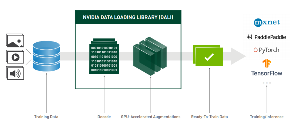
The NVIDIA Data Loading Library (DALI) is a library for data loading and pre-processing to accelerate deep learning applications. It provides a collection of highly optimized building blocks for loading and processing image, video, and audio data. DALI addresses the problem of the CPU bottleneck by offloading data preprocessing to the GPU. In addition, it offers some powerful features:
- DALI offers data processing primitives for a variety of deep learning applications. The supported input formats include most used image file formats.
- DALI relies on its own execution engine, built to maximize the throughput of the input pipeline.
- It can be used as a portable drop-in replacement for built-in data loaders and data iterators in popular deep learning frameworks.
- Features such as prefetching, parallel execution, and batch processing are handled transparently for the user.
- Different deep learning frameworks have multiple data pre-processing implementations, resulting in challenges such as portability of training and inference workflows, and code maintainability. Data processing pipelines implemented using DALI are portable because they can easily be retargeted to TensorFlow, PyTorch, MXNet and PaddlePaddle.
- Often the pre-processing routines that are used for inference are like the ones used for training, therefore implementing both using the same tools can save you some boilerplate and code repetition.
Install DALI: https://developer.nvidia.com/dali-download-page (Req: Linux x64; CUDA9.0+; TF1.7+ / Pytorch 0.4)
At the core of data processing with DALI lies the concept of a data processing
pipeline. It is composed of multiple operations connected in a directed graph and contained in an object of classnvidia.dali.Pipeline. This class provides functions necessary for defining, building, and running data processing pipelines.Those special operators act like a data source – readers, random number generators and external source fall into this category.
DALI offers CPU and GPU implementations for a wide range of processing operators. The availability of a CPU or GPU implementation depends on the nature of the operator. Make sure to check the documentation for an up-to-date list of supported operations, as it is expanded with every release.
The easiest way to define a DALI pipeline is using the pipeline_def Python decorator. To create a pipeline, we define a function where we instantiate and connect the desired operators and return the relevant outputs. Then just decorate it with pipeline_def. Let's start with defining a very simple pipeline, which will have two operators.
Let's start with defining a very simple pipeline, which will have two operators. The first operator is a file reader that discovers and loads files contained in a directory. The reader outputs both the contents of the files (in this case, PNGs) and the labels, which are inferred from the directory structure. The second operator is an image decoder. Lastly, we return the image and label pairs.
In the simple_pipeline function we define the operations to be performed and the flow of the computation between them. For more information about pipeline_def look to the documentation.
batch_size=4

@pipeline_def
def simple_pipeline():
    # use fn.readers.file to read encoded images and labels from the hard drive
    pngs, labels=fn.readers.file(file_root=image_dir)
    # use the fn.decoders.image operation to decode images from png to RGB
    images=fn.decoders.image(pngs, device='cpu')
    # specify which of the intermediate variables should be returned as the outputs of the pipeline
    return images, labels
Notice that decorating a function with pipeline_def adds new named arguments to it. They can be used to control various aspects of the pipeline, such as batch size, number of threads used to perform computation on the CPU, and which GPU device to use (though pipeline created with simple_pipeline does not yet use GPU for compute). For more information about Pipeline arguments you can look to Pipeline documentation.
Once built, a pipeline instance runs in an asynchronous fashion by calling the pipeline's run() method to get a batch of results. We unpack the results into images and labels as expected. Both of these elements contain a list of tensors.
In order to see the images, we will need to loop over all tensors contained in TensorList, accessed with its at method.
# define a function display images
def show_images(image_batch):
    columns=4
    rows=1
    # create plot
    fig=plt.figure(figsize=(15, (15 // columns) * rows))
    gs=gridspec.GridSpec(rows, columns)
    for idx in range(rows*columns):
        plt.subplot(gs[idx])
        plt.axis("off")
        plt.imshow(image_batch.at(idx))
    plt.tight_layout()

show_images(images)Deep learning models require training with vast amounts of data to achieve accurate results. DALI can not only read images from disk and batch them into tensors, it can also perform various augmentations on those images to improve deep learning training results. Data augmentation artificially increases the size of a data set by introducing random disturbances to the data, such as geometric deformations, color transforms, noise addition, and so on. These disturbances help produce models that are more robust in their predictions, avoid overfitting, and deliver better accuracy. We will use DALI to demonstrate data augmentation that we will introduce for model training, such as cropping, resizing, and flipping.
import random

@pipeline_def
def augmentation_pipeline():
    # use fn.readers.file to read encoded images and labels from the hard drive
    image_pngs, _=fn.readers.file(file_root=image_dir)
    # use the fn.decoders.image operation to decode images from png to RGB
    images=fn.decoders.image(image_pngs, device='cpu')

    # the same augmentation needs to be performed on the associated masks
    mask_pngs, _=fn.readers.file(file_root=mask_dir)
    masks=fn.decoders.image(mask_pngs, device='cpu')

    image_size=512
    roi_size=image_size*.5
    roi_start_x=image_size*random.uniform(0, 0.5)
    roi_start_y=image_size*random.uniform(0, 0.5)

    # use fn.resize to investigate an roi, region of interest
    resized_images=fn.resize(images, size=[512, 512], roi_start=[roi_start_x, roi_start_y], roi_end=[roi_start_x+roi_size, roi_start_y+roi_size])
    resized_masks=fn.resize(masks, size=[512, 512], roi_start=[roi_start_x, roi_start_y], roi_end=[roi_start_x+roi_size, roi_start_y+roi_size])

    # use fn.resize to flip the image
    flipped_images=fn.resize(images, size=[-512, -512])
    flipped_masks=fn.resize(masks, size=[-512, -512])
    return images, resized_images, flipped_images, masks, resized_masks, flipped_masks

pipe=augmentation_pipeline(batch_size=batch_size, num_threads=4, device_id=0)
pipe.build()
augmentation_pipe_output=pipe.run()

# define a function display images
def show_augmented_images(pipe_output):
    image_batch, resized_image_batch, flipped_image_batch, mask_batch, resized_mask_batch, flipped_mask_batch=pipe_output
    columns=6
    rows=batch_size
    # create plot
    fig=plt.figure(figsize=(15, (15 // columns) * rows))
    gs=gridspec.GridSpec(rows, columns)
    grid_data=[image_batch, resized_image_batch, flipped_image_batch, mask_batch, resized_mask_batch, flipped_mask_batch]
    grid=0
    for row_idx in range(rows):
        for col_idx in range(columns):
            plt.subplot(gs[grid])
            plt.axis('off')
            plt.imshow(grid_data[col_idx].at(row_idx))
            grid+=1
    plt.tight_layout()

show_augmented_images(augmentation_pipe_output)
Now let us perform additional data augmentation by as rotating each image (by a random angle). To generate a random angle, we can use random.uniform, and rotate for the rotation. We create another pipeline that uses the GPU to perform augmentations. DALI makes this transition very easy. The only thing that changes is the definition of the rotate operator. We only need to set the device argument to gpu and make sure that its input is transferred to the GPU by calling .gpu().
Keep in mind that the resulting images are also allocated in the GPU memory, which is typically what we want, since the model requires the data in GPU memory. In any case, copying back the data to CPU memory after running the pipeline can be easily achieved by calling as_cpu on the objects returned by Pipeline.run().
@pipeline_def
def rotate_pipeline():
    images, _=fn.readers.file(file_root=image_dir)
    masks, _=fn.readers.file(file_root=mask_dir)
    images=fn.decoders.image(images, device='cpu')
    masks=fn.decoders.image(masks, device='cpu')

    angle=fn.random.uniform(range=(-30.0, 30.0))
    rotated_images = fn.rotate(images.gpu(), angle=angle, fill_value=0, keep_size=True, device='gpu')
    rotated_masks = fn.rotate(masks.gpu(), angle=angle, fill_value=0, keep_size=True, device='gpu')

    return rotated_images, rotated_masks

pipe=rotate_pipeline(batch_size=batch_size, num_threads=4, device_id=0)
pipe.build()
rotate_pipe_output= pipe.run()file: 02_efficient_model_training.ipynb
- 32 GB system RAM
- 32 GB of GPU RAM
- 8 core CPU
- 1 NVIDIA GPU
- 100 GB of SSD space
In this notebook, you will learn how to train a segmentation model with the TAO Toolkit using pre-trained Resnet-18 weights. In addition, you will learn how to export the model for deployment.
It lets developers fine-tune pretrained models with custom data to produce highly accurate computer vision models efficiently, eliminating the need for large training runs and deep AI expertise. In addition, it also enables model optimization for inference performance.

YouTube: https://youtu.be/vKKCSMfE05A
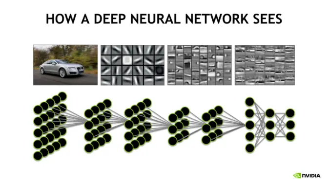
In practice, it is rare and inefficient to initiate the learning task on a network with randomly initialized weights due to factors like data scarcity (inadequate number of training samples) or prolonged training times. One of the most common techniques to overcome this is to use transfer learning. Transfer learning is the process of transferring learned features from one application to another. developers use a model trained on one task and re-train to use it on a different task. This works surprisingly well as many of the early layers in a neural network are the same for similar tasks.
For example, many of the early layers in a convolutional neural network used for a Computer Vision (CV) model are primarily used to identify outlines, curves, and other features in an image. The network formed by these layers are referred to as the backbone of a more complex model. Also known as feature extractors, they take as input the image and extracts the feature map upon which the rest of the network is based. The learned features from these layers can be applied to similar tasks carrying out the same identification in other domains. Transfer learning enables adaptation (fine-tuning) of an existing neural network to a new one, which requires significantly less domain-specific data.
More information about transfer learning can be found in this Nvidia blogpost.
Developers, system builders, and software partners building disaster risk monitoring systems can bring their own custom data to train with and fine-tune pre-trained models quickly instead of going through significant effort in large data collection and training from scratch. General purpose vision models provide pre-trained weights for popular network architectures to train an image classification model, an object detection model, or a segmentation model. This gives users the flexibility and control to build AI models for any number of applications, from smaller lightweight models for edge deployment to larger models for more complex tasks. They are trained on Open Images data set and provide a much better starting point for training versus training from scratch or starting from random weights.
When working with TAO, first choose the model architecture to be built, then choose one of the supported backbones.
Note: The pre-trained weights from each feature extraction network merely act as a starting point and may not be used without re-training. In addition, the pre-trained weights are network specific and shouldn't be shared across models that use different architectures.
| Image Classification | Object detection - DetectNet_V2 | Object detection - FasterRCNN | Object detection - SSD | Object detection - YOLOV3 | Object detection - YOLOV4 | Object detection - RetinaNet | Object detection - DSSD | Segmentation - MaskRCCN | Segmentation - Unet | |
|---|---|---|---|---|---|---|---|---|---|---|
| ResNet10/18/34/50/101 | OK | OK | OK | OK | OK | OK | OK | OK | OK | OK |
| VGG16/19 | OK | OK | OK | OK | OK | OK | OK | OK | OK | |
| GoogLeNet | OK | OK | OK | OK | OK | OK | OK | OK | ||
| MobileNet | V1/V2 | OK | OK | OK | OK | OK | OK | OK | OK | |
| SqueezeNet | OK | OK | OK | OK | OK | OK | OK | |||
| DarkNet19/53 | OK | OK | OK | OK | OK | OK | OK | OK | ||
| CSPDarkNet19/53 | OK | OK | ||||||||
| EfficientnetB0 | OK | OK | OK | OK | OK |
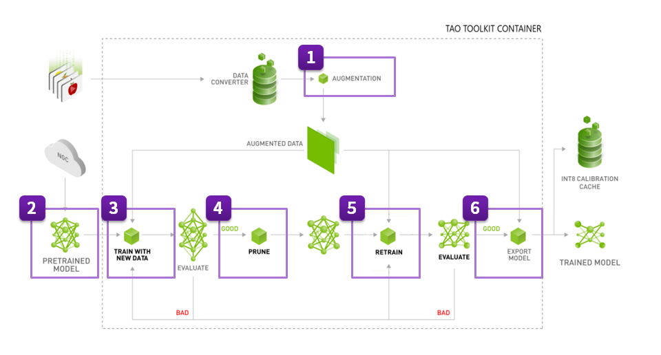
Building disaster risk monitoring systems is hard. And tailoring even a single component to the needs of the enterprise for deployment is even harder. Deployment for a domain-specific application typically requires several cycles of re-training, fine-tuning, and deploying the model until it satisfies the requirements. As a starting point, training typically follows the below steps:
- Configuration
- Download a pre-trained model from NGC
- Prepare the data for training
- Train the model using transfer learning
- Evaluate the model for target predictions
- Export the model
- Steps to optimize the model for improved inference performance
Moore in Computer Vision in production –Nvidia DeepStream on medium blogpost
The TAO Toolkit is a zero-coding framework that makes it easy to get started. It uses a launcher to pull from NGC registry and instantiate the appropriate TAO container that performs the desired subtasks such as convert data, train, evaluate, or export. The TAO launcher is a python package distributed as a python wheel listed in the nvidia-pyindex python index, which has been prepared for you already. Users interact with the launcher with its Command Line Interface that is configured using simple Protocol Buffer specification files to include parameters such as the data set parameters, model parameters, and optimizer and training hyperparameters. More information about the TAO Toolkit Launcher can be found in the TAO Docs.
The tasks can be invoked from the TAO Toolkit Launcher using the convention tao <task> <subtask> <args_per_subtask>, where <args_per_subtask> are the arguments required for a given subtask. Once the container is launched, the subtasks are run by the TAO Toolkit containers using the appropriate hardware resources.
To see the usage of different functionality that are supported, use the -h or --help option. For more information, see the TAO Toolkit Quick Start Guide.
With the TAO Toolkit, users can train models for object detection, classification, segmentation, optical character recognition, facial landmark estimation, gaze estimation, and more. In TAO's terminology, these would be the tasks, which support subtasks such as train, prune, evaluate, export, etc. ach task/subtask requires different combinations of configuration files to accommodate for different parameters, such as the dataset parameters, model parameters, and optimizer and training hyperparameters. hey are detailed in the Getting Started Guide for reference. It's very helpful to have these resources handy when working with the TAO Toolkit.
get help with !tao <task> <subtask> --help
!tao mask_rcnn prune --help

~/.tao_mounts.json wasn't found. Falling back to obtain mount points and docker configs from ~/.tlt_mounts.json.
Please note that this will be deprecated going forward.
2022-08-03 20:06:38,820 [INFO] root: Registry: ['nvcr.io']
2022-08-03 20:06:38,977 [INFO] tlt.components.instance_handler.local_instance: Running command in container: nvcr.io/nvidia/tao/tao-toolkit-tf:v3.21.11-tf1.15.5-py3
2022-08-03 20:06:38,984 [INFO] root: No mount points were found in the /root/.tlt_mounts.json file.
2022-08-03 20:06:38,984 [WARNING] tlt.components.docker_handler.docker_handler:
Docker will run the commands as root. If you would like to retain your
local host permissions, please add the "user":"UID:GID" in the
DockerOptions portion of the "/root/.tlt_mounts.json" file. You can obtain your
users UID and GID by using the "id -u" and "id -g" commands on the
terminal.
Using TensorFlow backend.
usage: mask_rcnn prune [-h] [--num_processes NUM_PROCESSES] [--gpus GPUS]
                       [--gpu_index GPU_INDEX [GPU_INDEX ...]] [--use_amp]
                       [--log_file LOG_FILE] -m MODEL -o OUTPUT_DIR -k KEY
                       [-n NORMALIZER] [-eq EQUALIZATION_CRITERION]
                       [-pg PRUNING_GRANULARITY] [-pth PRUNING_THRESHOLD]
                       [-nf MIN_NUM_FILTERS]
                       [-el [EXCLUDED_LAYERS [EXCLUDED_LAYERS ...]]] [-v]
                       {evaluate,export,inference,inference_trt,prune,train}
                       ...

optional arguments:
  -h, --help            show this help message and exit
  --num_processes NUM_PROCESSES, -np NUM_PROCESSES
                        The number of horovod child processes to be spawned.
                        Default is -1(equal to --gpus).
  --gpus GPUS           The number of GPUs to be used for the job.
  --gpu_index GPU_INDEX [GPU_INDEX ...]
                        The indices of the GPU's to be used.
  --use_amp             Flag to enable Auto Mixed Precision.
  --log_file LOG_FILE   Path to the output log file.
  -m MODEL, --model MODEL
                        Path to the target model for pruning
  -o OUTPUT_DIR, --output_dir OUTPUT_DIR
                        Output directory for pruned model
  -k KEY, --key KEY     Key to load a .tlt model
  -n NORMALIZER, --normalizer NORMALIZER
                        `max` to normalize by dividing each norm by the
                        maximum norm within a layer; `L2` to normalize by
                        dividing by the L2 norm of the vector comprising all
                        kernel norms. (default: `max`)
  -eq EQUALIZATION_CRITERION, --equalization_criterion EQUALIZATION_CRITERION
                        Criteria to equalize the stats of inputs to an element
                        wise op layer. Options are [arithmetic_mean,
                        geometric_mean, union, intersection]. (default:
                        `union`)
  -pg PRUNING_GRANULARITY, --pruning_granularity PRUNING_GRANULARITY
                        Pruning granularity: number of filters to remove at a
                        time. (default:8)
  -pth PRUNING_THRESHOLD, --pruning_threshold PRUNING_THRESHOLD
                        Threshold to compare normalized norm against
                        (default:0.1)
  -nf MIN_NUM_FILTERS, --min_num_filters MIN_NUM_FILTERS
                        Minimum number of filters to keep per layer.
                        (default:16)
  -el [EXCLUDED_LAYERS [EXCLUDED_LAYERS ...]], --excluded_layers [EXCLUDED_LAYERS [EXCLUDED_LAYERS ...]]
                        List of excluded_layers. Examples: -i item1 item2
  -v, --verbose         Include this flag in command line invocation for
                        verbose logs.

tasks:
  {evaluate,export,inference,inference_trt,prune,train}
2022-08-03 20:06:42,764 [INFO] tlt.components.docker_handler.docker_handler: Stopping container.
U-Net is a network for image segmentation. This is the type of task we want to perform for our disaster risk monitoring system in order to label each pixel as either flood or notflood. With the TAO Toolkit, we can choose the desired ResNet-18 backbone as a feature extractor. As such, we will use the unet task, which supports the following subtasks:
trainevaluateinferencepruneexport
These subtasks can be invoked using the convention tao unet <subtask> <args_per_subtask> on the command-line, where args_per_subtask are the arguments required for a given subtask.
For the remaining of the lab, we will use the TAO Toolkit to train a semantic segmentation model. Below is what the model development workflow looks like. We start by preparing a pre-trained model and the data. Next, we prepare the configuration file(s) and begin to train the model with new data and evaluate its performance. We will export the model once its satisfactory. Note that this notebook does not include inference optimization steps, which is important for disaster risk monitoring systems that are deployed on edge devices.
Pre-trained model -> Prepare data -> Train w/ Spec File -> Evaluate -> Export Model
We set up a couple of environment variables to help us mount the local directories to the tao container. Specifically, we want to set paths for the $LOCAL_TRAINING_DATA, $LOCAL_SPEC_DIR, and $LOCAL_PROJECT_DIR for the output of the TAO experiment with their respective paths in the TAO container. In doing so, we can make sure that the TAO experiment generated collaterals such as checkpoints, model files (e.g. .tlt or .etlt), and logs are output to $LOCAL_PROJECT_DIR/unet.
Note that users will be able to define their own export encryption key when training from a general-purpose model. This is to protect proprietary IP and used to decrypt the .etlt model during deployment.
The cell below maps the project directory on your local host to a workspace directory in the TAO docker instance, so that the data and the results are mapped from in and out of the docker. This is done by creating a .tao_mounts.json file. For more information, please refer to the launcher instance
# mapping up the local directories to the TAO docker
import json
mounts_file = os.path.expanduser("~/.tao_mounts.json")

drive_map = {
    "Mounts": [
            # Mapping the data directory
            {
                "source": os.environ["LOCAL_PROJECT_DIR"],
                "destination": "/workspace/tao-experiments"
            },
            # Mapping the specs directory.
            {
                "source": os.environ["LOCAL_SPECS_DIR"],
                "destination": os.environ["TAO_SPECS_DIR"]
            },
            # Mapping the data directory.
            {
                "source": os.environ["LOCAL_DATA_DIR"],
                "destination": os.environ["TAO_DATA_DIR"]
            },
        ],
    "DockerOptions": {
        "user": "{}:{}".format(os.getuid(), os.getgid())
    }
}

# writing the mounts file
with open(mounts_file, "w") as mfile:
json.dump(drive_map, mfile, indent=4)Developers typically begin by choosing and downloading a pre-trained model from NGC which contains pre-trained weights of the architecture of their choice. It's difficult to immediately identify which model/architecture will work best for a specific use case as there is often a tradeoff between time to train, accuracy, and inference performance. It is common to compare across multiple models before picking the best candidate.
Here are some pointers that will help choose an appropriate model:
- Look at the model inputs/outputs
- Input format is also an important consideration. For example, some models expect the input to be 0-1 normalized with input channels in RGB order.
We can use the ngc registry model list <model_glob_string> command to get a list of models that are hosted on the NGC model registry. For example, we can use ngc registry model list nvidia/tao/* to list all available models. The --column option identifies the columns of interest. More information about the NGC Registry CLI can be found in the User Guide. The ngc registry model download-version <org>/[<team>/]<model-name:version> command will download the model from the registry. It has a --dest option to specify the path to download directory.
The TAO Toolkit expects the training data for the unet task to be in the format described in the documentation. unet expects the images and corresponding masks encoded as images. Each mask image is a single-channel image, where every pixel is assigned an integer value that represents the segmentation class. Additionally, each image and label have the same file ID before the extension. The image-to-label correspondence is maintained using this filename.
Training configuration is done through a training spec file, which includes options such as which data set to use for training, which data set to use for validation, which pre-trained model architecture to use, which hyperparameters to tune, and other training options. The train, evaluate, prune, and inference subtasks for an U-Net experiment share the same configuration file. Configuration files can be created from scratch or modified using the templates provided in TAO Toolkit's sample applications.
The training configuration file has eight sections:
dataset_configmodel_configtraining_config
The dataloader defines the path to the data to be trained on and the class mapping for the classes in the data set. We have previously generated images and masks for the training data sets. To use the newly generated training data, update the dataset_config parameter in the spec file to reference the correct directory.
dataset (str): The input type dataset used. The currently supported dataset iscustomto the user. Open-source datasets will be added in the future.augment (bool): If the input should augmented online while training. When using one’s own data set to train and fine-tune a model, the data set can be augmented while training to introduce variations in the data set. This is known as online augmentation. This is very useful in training as data variation improves the overall quality of the model and prevents overfitting. Training a deep neural network requires large amounts of annotated data, which can be a manual and expensive process. Furthermore, it can be difficult to estimate all the corner cases that the network may go through. The TAO Toolkit provides spatial augmentation (resize and flip) and color space augmentation (brightness) to create synthetic data variations.augmentation_config (dict):spatial_augmentation (dict): Supports spatial augmentation such as flip, zoom, and translate.hflip_probability (float): Probability to flip an input image horizontally.vflip_probability (float): Probability to flip an input image vertically.crop_and_resize_prob (float)
brightness_augmentation (dict): Configures the color space transformation.delta (float): Adjust brightness using delta value.
input_image_type (str): The input image type to indicate if input image isgrayscaleorcolor(RGB).train_images_path (str),train_masks_path (str),val_images_path (str),val_masks_path (str),test_images_path (str): The path string for train images, train masks, validation images, validation masks, and test images (optional).data_class_config (dict): Proto dictionary that contains information of training classes as part of target_classes proto which is described below.target_classes (dict): The repeated field for every training class. The following are required parameters for the target_classes config:name (str): The name of the target class.mapping_class (str): The name of the mapping class for the target class. If the class needs to be trained as is, then name and mapping_class should be the same.label_id (int): The pixel that belongs to this target class is assigned this label_id value in the mask image.
Note the supported image extension formats for training images are “.png”, “.jpg”, “.jpeg”, “.PNG”, “.JPG”, and “.JPEG”.
dataset_config {
  dataset: "custom"
  augment: True
  augmentation_config {
    spatial_augmentation {
      hflip_probability : 0.5
      vflip_probability : 0.5
      crop_and_resize_prob : 0.5
    }
  }
  input_image_type: "color"
  train_images_path:"/workspace/tao-experiments/data/images/train"
  train_masks_path:"/workspace/tao-experiments/data/masks/train"

  val_images_path:"/workspace/tao-experiments/data/images/val"
  val_masks_path:"/workspace/tao-experiments/data/masks/val"

  test_images_path:"/workspace/tao-experiments/data/images/val"

  data_class_config {
    target_classes {
      name: "notflood"
      mapping_class: "notflood"
      label_id: 0
    }
    target_classes {
      name: "flood"
      mapping_class: "flood"
      label_id: 255
    }
  }
}
The segmentation model can be configured using the model_config option in the spec file.
all_projections (bool): For templates with shortcut connections, this parameter defines whether all shortcuts should be instantiated with 1x1 projection layers, irrespective of a change in stride across the input and output.arch (str): The architecture of the backbone feature extractor to be used for training.num_layers (int): The depth of the feature extractor for scalable templates.use_batch_norm (bool): A Boolean value that determines whether to use batch normalization layers or not.training_precision (dict): Contains a nested parameter that sets the precision of the back-end training framework.backend_floatx: The back-end training framework should be set toFLOAT322.
initializer (choice): Initialization of convolutional layers. Supported initializations areHE_UNIFORM,HE_NORMAL, andGLOROT_UNIFORM.model_input_height (int): The model input height dimension of the model, which should be a multiple of 16.model_input_width (int): The model input width dimension of the model, which should be a multiple of 16.model_input_channels (int): The model-input channels dimension of the model, which should be set to 3 for a Resnet/VGG backbone.
model_config {
  model_input_width: 512
  model_input_height: 512
  model_input_channels: 3
  num_layers: 18
  all_projections: True
  arch: "resnet"
  use_batch_norm: False
  training_precision {
    backend_floatx: FLOAT32
  }
}
########## LEAVE NEW LINE BELOW
The training_config describes the training and learning process.
batch_size (int): The number of images per batch per gpu.epochs (int): The number of epochs to train the model. One epoch represents one iteration of training through the entire dataset.log_summary_steps (int): The summary-steps interval at which train details are printed to stdout.checkpoint_interval (int): The number of epochs interval at which the checkpoint is saved.loss (str): The loss to be used for segmentation.learning_rate (float): The learning-rate initialization value.regularizer (dict): This parameter configures the type and weight of the regularizer to be used during training. The two parameters include:type (Choice): The type of the regularizer being used should beL2orL1.weight (Float): The floating-point weight of the regularizer.
optimizer (dict): This parameter defines which optimizer to use for training, and the parameters to configure it, namely:adam:epsilon (float): Is a very small number to prevent any division by zero in the implementation.beta1 (float).beta2 (float).
activation (str): The activation to be used on the last layer supported issoftmax.
training_config {
  batch_size: 1
  epochs: 30
  log_summary_steps: 10
  checkpoint_interval: 10
  loss: "cross_dice_sum"
  learning_rate: 0.0001
  regularizer {
    type: L2
    weight: 2e-5
  }
  optimizer {
    adam {
      epsilon: 9.99999993923e-09
      beta1: 0.899999976158
      beta2: 0.999000012875
    }
  }
}
After preparing input data and setting up a spec file. You are now ready to start training a semantic segmentation network.
tao unet train [-h] -e <EXPERIMENT_SPEC_FILE>
                    -r <RESULTS_DIR>
                    -n <MODEL_NAME>
                    -m <PRETRAINED_MODEL_FILE>
                    -k <key>
                    [-v Set Verbosity of the logger]
                    [--gpus GPUS]
                    [--gpu_index GPU_INDEX]
When using the train subtask, the -e argument indicates the path to the spec file, the -r argument indicates the result directory, and the -k indicates the key to load the pre-trained weights. There are some optional arguments that might be useful such as -n to indicates the name of the final step model saved and -m to indicate the path to a pre-trained model to initialize.
Multi-GPU support can be enabled for those with the hardware using the --gpus argument. When running the training with more than one GPU, we will need to modify the batch_size and learning_rate. In most cases, scaling down the batch-size by a factor of NUM_GPU's or scaling up the learning rate by a factor of NUM_GPUs would be a good place to start.
Once we are satisfied with our model, we can move to deployment. unet includes an export subtask to export and prepare a trained U-Net model for deployment. Exporting the model decouples the training process from deployment and allows conversion to TensorRT engines outside the TAO environment. TensorRT engines are specific to each hardware configuration and should be generated for each unique inference environment. This may be interchangeably referred to as the .trt or .engine file. The same exported TAO model may be used universally across training and deployment hardware. This is referred to as the .etlt file, or encrypted TAO file.
NVIDIA TensorRT is a platform for high-performance deep learning inference. It includes a deep learning inference optimizer and runtime that delivers low latency and high throughput for deep learning inference applications. TensorRT-based applications perform up to 40x faster than CPU-only platforms during inference.
With TensorRT, you can optimize neural network models trained in all major frameworks, calibrate for lower precision with high accuracy, and finally deploy to hyperscale data centers, embedded, or automotive product platforms.
Here are some great resources to learn more about TensorRT:
- Main Page: https://developer.nvidia.com/tensorrt
- Blogs: https://devblogs.nvidia.com/speed-up-inference-tensorrt/
- Download: https://developer.nvidia.com/nvidia-tensorrt-download
- Documentation: https://docs.nvidia.com/deeplearning/sdk/tensorrt-developer-guide/index.html
- Sample Code: https://docs.nvidia.com/deeplearning/sdk/tensorrt-sample-support-guide/index.html
- GitHub: https://github.com/NVIDIA/TensorRT
- NGC Container: https://ngc.nvidia.com/catalog/containers/nvidia:tensorrt
When using the export subtask, the -m argument indicates the path to the .tlt model file to be exported, the -e argument indicates the path to the spec file, and -k argument indicates the key to load the model. There are two optional arguments, --gen_ds_config and --engine_file that are useful for us. The --gen_ds_config argument indicates whether to generate a template inference configuration file as well as a label file. The --engine_file indicates the path to the serialized TensorRT engine file.
Note that the TensorRT file is hardware specific and cannot be generalized across GPUs. Since a TensorRT engine file is hardware specific, you cannot use an engine file for deployment unless the deployment GPU is identical to the training GPU. This is true in our case since the Triton Inference Server will be deployed from the same hardware.
file: 03_model_deployment_for_inference.ipynb
NVIDIA Triton Inference Server simplifies the deployment of AI models at scale in production. Triton is an open-source, inference-serving software that lets teams deploy trained AI models from any framework, from local storage, or from Google Cloud Platform or Azure on any GPU or CPU-based infrastructure, cloud, data center, or edge. The below figure shows the Triton Inference Server high-level architecture. The model repository is a file-system based repository of the models that Triton will make available for inferencing. Inference requests arrive at the server via either HTTP/REST, gRPC, or by the C API and are then routed to the appropriate per-model scheduler. Triton implements multiple scheduling and batching algorithms that can be configured on a model-by-model basis. Each model's scheduler optionally performs batching of inference requests and then passes the requests to the backend corresponding to the model type. The backend performs inferencing using the inputs provided in the batched requests to produce the requested outputs. The outputs are then returned.
Setting up the Triton Inference Server requires software for the server and the client. One can get started with Triton Inference Server by pulling the container from the NVIDIA NGC catalog. In this lab, we already have Triton Inference Server instance running. The code to run a Triton Server Instance is shown below. More details can be found in the QuickStart and build instructions:
We've also installed the Triton Inference Server Client libraries to provide APIs that make it easy to communicate with Triton from your C++ or Python application. Using these libraries, you can send either HTTP/REST or gRPC requests to Triton to access all its capabilities: inferencing, status and health, statistics and metrics, model repository management, etc. These libraries also support using system and CUDA shared memory for passing inputs to and receiving outputs from Triton. The easiest way to get the Python client library is to use pip to install the tritonclient module, as detailed below. For more details on how to download or build the Triton Inference Server Client libraries, you can find the documentation here, as well as examples that show the use of both the C++ and Python libraries.
pip install nvidia-pyindex
pip install tritonclient[all]
Triton Inference Server serves models within a model repository. When you first run Triton Inference Server, you'll specify the model repository where the models reside:
tritonserver --model-repository=/models
Each model resides in its own model subdirectory within the model repository - i.e., each directory within /models represents a unique model. For example, in this notebook we'll be deploying our flood_segmentation_model. All models typically follow a similar directory structure. Within each of these directories, we'll create a configuration file config.pbtxt that details information about the model - e.g. batch size, input shapes, deployment backend (PyTorch, ONNX, TensorFlow, TensorRT, etc.) and more. Additionally, we can create one or more versions of our model. Each version lives under a subdirectory name with the respective version number, starting with 1. It is within this subdirectory where our model files reside.
root@server:/models$ tree
.
├── flood_segmentation_model
│   ├── 1
│   │   └── model.plan
│   └── config.pbtxt
│
We can also add a file representing the names of the outputs. We have omitted this step in this notebook for the sake of brevity. For more details on how to work with model repositories and model directory structures in Triton Inference Server, please see the documentation. Below, we'll create the model directory structure for our flood detection segmentation model.
With our model directory set up, we now turn our attention to creating the configuration file for our model. A minimal model configuration must specify the name of the model, the platform and/or backend properties, the max_batch_size property, and the input and output tensors of the model (name, data type, and shape). We can get the output tensor name from the nvinfer_config.txt file we generated before under output-blob-names. For more details on how to create model configuration files within Triton Inference Server, please see the documentation.
With our model directory structures created, models defined and exported, and configuration files created, we will now wait for Triton Inference Server to load our models. We have set up this lab to use Triton Inference Server in polling mode. This means that Triton Inference Server will continuously poll for modifications to our models or for newly created models - once every 30 seconds. Please run the cell below to allow time for Triton Inference Server to poll for new models/modifications before proceeding. Due to the asynchronous nature of this step, we have added 15 seconds to be safe.
At this point, our models should be deployed and ready to use! To confirm Triton Inference Server is up and running, we can send a curl request to the below URL. The HTTP request returns status 200 if Triton is ready and non-200 if it is not ready. We can also send a curl request to our model endpoints to confirm our models are deployed and ready to use. Additionally, we will also see information about our models such:
- The name of our model,
- The versions available for our model,
- The backend platform (e.g., tensort_rt, pytorch_libtorch, onnxruntime_onnx),
- The inputs and outputs, with their respective names, data types, and shapes.
Triton itself does not do anything with your input tensors, it simply feeds them to the model. Same for outputs. Ensuring that the preprocessing operations used for inference are defined identically as they were when the model was trained is key to achieving high accuracy. In our case, we need to perform normalization and mean subtraction to produce the final float planar data to the TensorRT engine for inferencing. We can get the offsets and net-scale-factor from the nvinfer_config.txt file. The pre-processing function is:
y = net scale factor * (x-mean)
where:
- x is the input pixel value. It is an int8 with range [0,255].
- mean is the corresponding mean value, read either from the mean file or as offsets[c], where c is the channel to which the input pixel belongs, and offsets is the array specified in the configuration file. It is a float.
- net-scale-factor is the pixel scaling factor specified in the configuration file. It is a float.
- y is the corresponding output pixel value. It is a float.
Once deployed, the Triton Inference Server can be connected to front-end applications such as those that power https://www.balcony.io/, which provides an emergency management platform that has the ability to send messages to personal devices. In terms of making the model better, improving on metrics like Intersect-Over-Union (IoU) translates to accurate flood modeling, and coupled with a time-optimized solution aids in real-time disaster response and eventual climate action.
- more about the challenge at [ETCI 2021](https://nasa-impact.github.io/etci2021/]
- more about flood detection by AI in this blogpost: Jumpstart Your Machine Learning Satellite Competition Submission
files: /flood_detection_w_AI
@inproceedings{paul2021flood,
    title   = {Flood Segmentation on Sentinel-1 SAR Imagery with Semi-Supervised Learning},
    author  = {Sayak Paul and Siddha Ganju},
    year    = {2021},
    URL = {https://arxiv.org/abs/2107.08369},
    booktitle = {NeurIPS Tackling Climate Change with Machine Learning Workshop}
}
Other interesting related links: