This course is jointly launched by Huawei and Chongqing University of Posts and Telecommunications, and Dalian University of Technology,matching the HCIA-AI V3.0(Released on September 17, 2020). Through this course, you will systematically understand the AI development history, the Huawei Ascend AI system, the full-stack all-scenario AI strategy,and the algorithms related to traditional machine learning and deep learning; TensorFlow and MindSpore. HCIA-AI V1.0 will be offline on June 30, 2021.
This lesson below is not mine, the source and copyright are for Huawei.
Content list
- AI OverView
- Machine Learning Overview
- Deep Learning
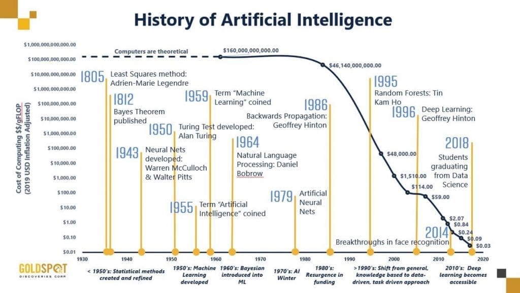
AI: A new technical science that focuses on there search and development of theories, methods, techniques, and application systems for simulating and extending human intelligence
Machine learning: A core research field of AI. It focuses on the study of how computers cano btain new knowledge or skills by simulating or performing learning behavior of human beings, and reorganize existing knowledge architecture to improve its performance.
Deep learning: Deep learning aims to simulate the human brain to interpret data such as images, sounds, and texts.
- The cognitive process of human beings is the process of inference and operation of various symbols.
- Human being is a physical symbol system, and so is a computer.
- The core of AI lies in knowledge representation, knowledge inference, and knowledge application. Knowledge and concepts can be represented with symbols. Cognition is the process of symbol processing while inference refers to the process of solving problems by using heuristic knowledge and search.
- The basis of thinking is neurons rather than the process of symbol processing
- Human brains vary from computers. A computer working mode based on connectionism is proposed to replace the computer working mode based on symbolic operation.
- Intelligence depends on perception and action.
- Intelligence requires no knowledge, representation, or inference. AI can evolve like human intelligence. Intelligent behavior can only be demonstrated in the real world through the constant interaction with the surrounding environment.
Holds that it is possible to create intelligent machines that can really reason and solve problems. Such machines are considered to be conscious and self-aware, can independently think about problems and work out optimal solutions to problems, have their own system of values and world views, and have all the same instincts as living things,
Holds that intelligent machines cannot really reason and solve problems. These machines only look intelligent, but do not have real intelligence.
- Application enablement: provides end-to-end services (ModelArts), layered APIs, and pre-integrated solutions
- MindSpore: supports the unified training and inference framework that is independent of the device, edge, and cloud
- provides automatic parallel capabilities. Can run a gorithms on dozens or even thousands of AI computing nodes with only a few lines of description.
- CANN: (Compute Architecture for Neural Networks) a chip operator library and highly automated operator development tool.
- A chip operators library and highly automated operator development toolkitOptimal development efficiency, in-depth optimization of the common operator library, and abundant APIs
- Ascend: provides a series of NPU IPs and chips based on a unified, scalable architecture.
- Atlas: enables an all-scenario AI infrastructure solution that is oriented to the device, edge, and cloud based on the Ascend series AI processors and various product forms.
Algorithmic biases are mainly caused by data biases.
- Tensorflow2.0: TensorFlow 2.0 has been officially released. It integrates Keras as its high-level API, greatly improving usability.
Machine learning is a core research field of AI, and it is also a necessary knowledge for deep learning.
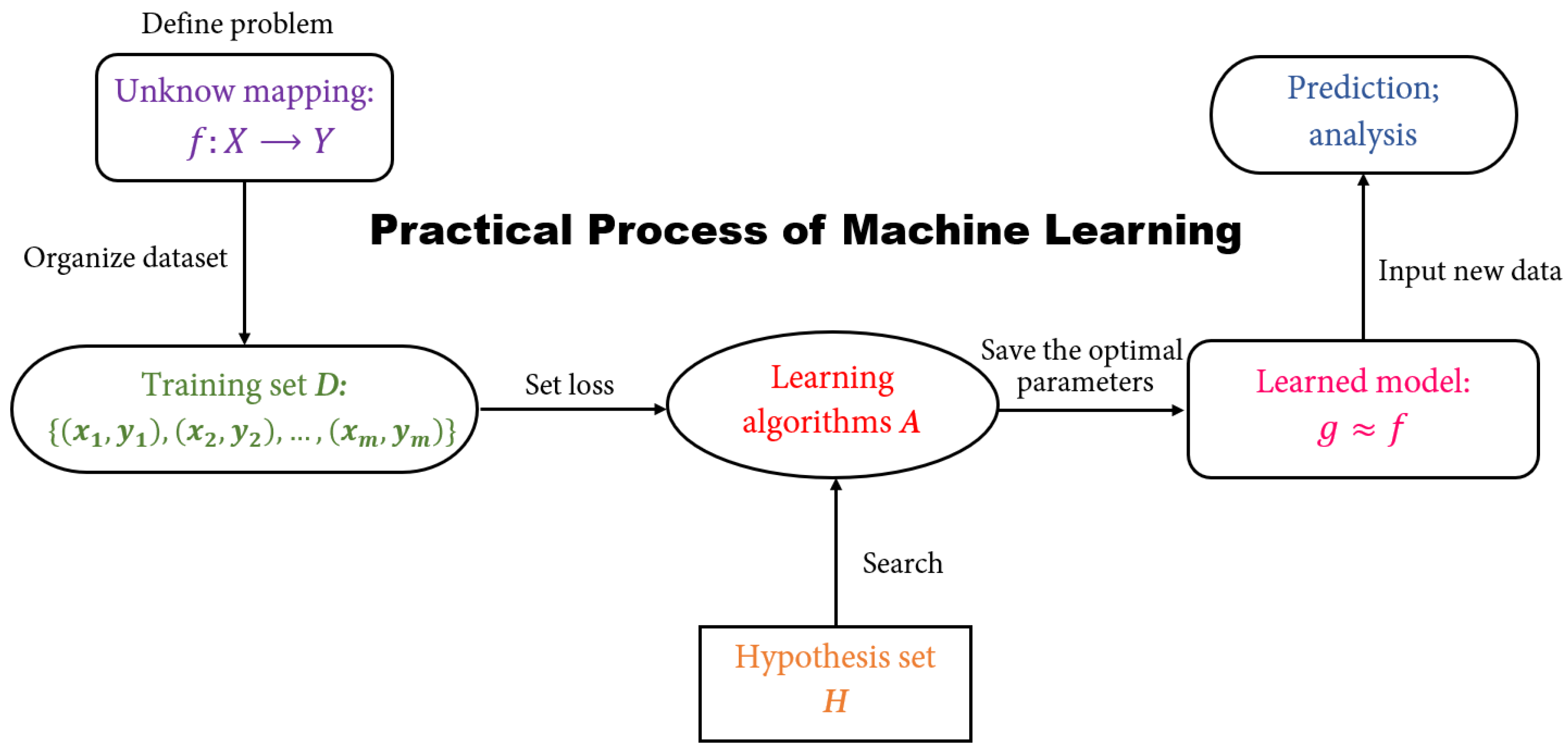
Machine learning (including deep learning) is a study of learning algorithms. A computer program is said to learn from experience 𝐸 with respect to some class of tasks 𝑇 and performance measure 𝑃 if its performance at tasks in 𝑇, as measured by 𝑃, improves with experience 𝐸.

Machine learning can deal with:
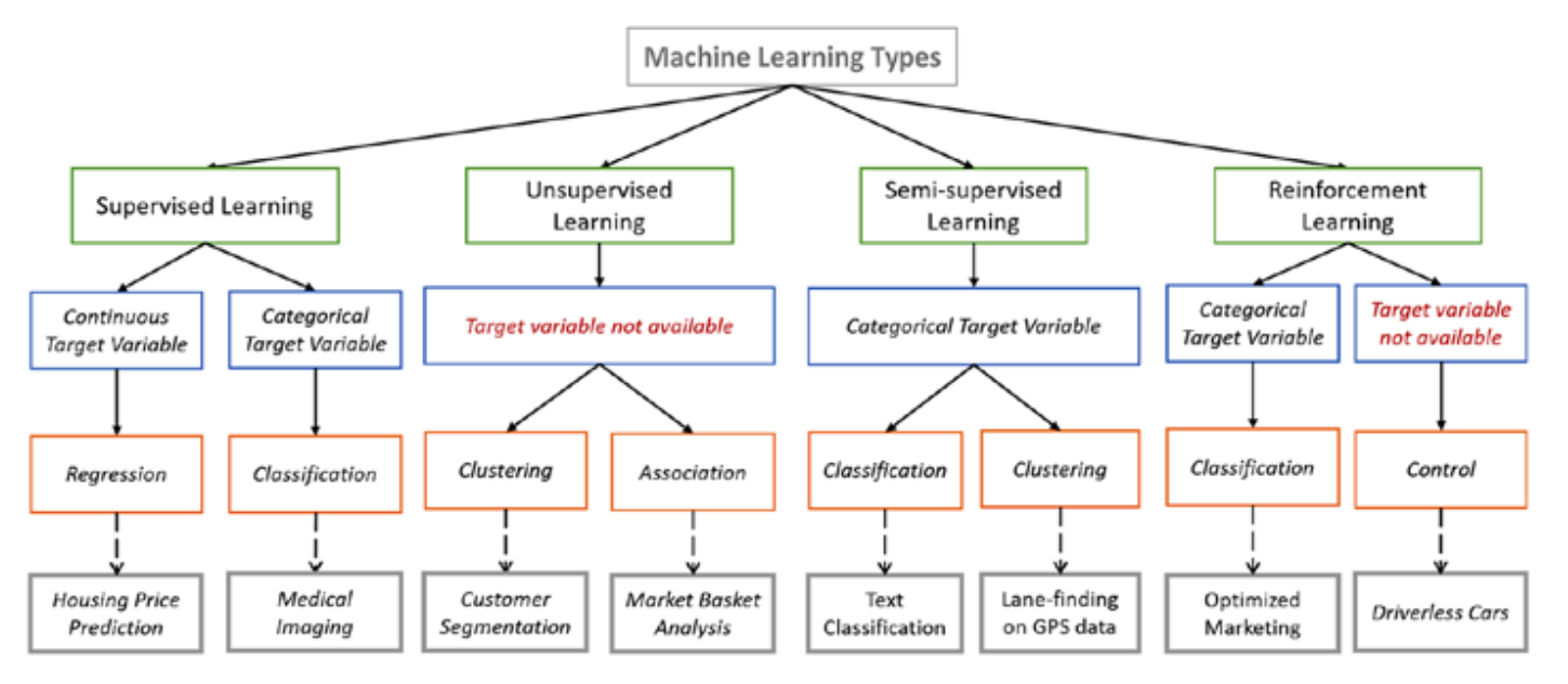
- assification: computer program needs to specify which of the k categories some input belongs to. To accomplish this task, learning algorithms usually output a function 𝑓:𝑅^𝑛 → (1,2,…,𝑘). For example, the image classification algorithm in computer vision is developed to handle classification tasks
- Regression: For this type of task, a computer program predicts the output for the given input. Learning algorithms typically output a function 𝑓:𝑅^𝑛 → 𝑅. An example of this task type is to predict the claim amount of an insured person (to set the insurance premium) or predict the security price
- lustering: A large amount of data from an unlabeled dataset is divided into multiple categories according to internal similarity of the data. Data in the same category is more similar than that in different categories. This feature can be used in scenarios such as image retrieval and user profile management
Obtain an optimal model with required performance through training and learning based on the samples of known categories. Then, use the model to map all inputs to outputs and check the output for the purpose of classifying unknown data.
- How much will I benefit from the stock next week?
- What's the temperature on Tuesday?
- Will there be a traffic jam on XX road during the morning rush hour tomorrow?
- Which method is more attractive to customers: 5 yuan voucher or 25% off?

For unlabeled samples, the learning algorithms directly model the input datasets. Clustering is a common form of unsupervised learning. We only need to put highly similar samples together, calculate the similarity between new samples and existing ones, and classify them by similarity.
- *Which audiences like to watch movies of the same subject? *
- Which of these components are damaged in a similar way?

In one task, a machine learning model that automatically uses a large amount of unlabeled data to assist learning directly of a small amount of labeled data.
- the labaled data predict a high temperature, but this can be because other complications, and we can decide which is true
Dinamic programing for interacting the enviroment.
always looks for best behaviors
Reinforcement learning is targeted at machines or robots.
*Autopilot: Should it brake or accelerate when the yellow light starts to flash? *
Cleaning robot: Should it keep working or go back for charging?
- Each data record is called a sample
- events that reflect the performance or nature of a sample in particular aspects are called features
- each sample is referred to as a training sample
- creating model from data = learning
- the process of using the model obtained after learning for prediction
- each sample is called a test sample
- more: https://forum.huawei.com/enterprise/en/important-concepts-of-machine-learning/thread/700585-893?from=latestPostsReplies
- Before using the data, you need to preprocess the data. There is no standard process for data preprocessing. Data preprocessing varies according to tasks and data set attributes. Common data preprocessing processes include removing unique attributes, processing missing values, encoding attributes, standardizing and regularizing data, selecting features, and analyzing principal components.
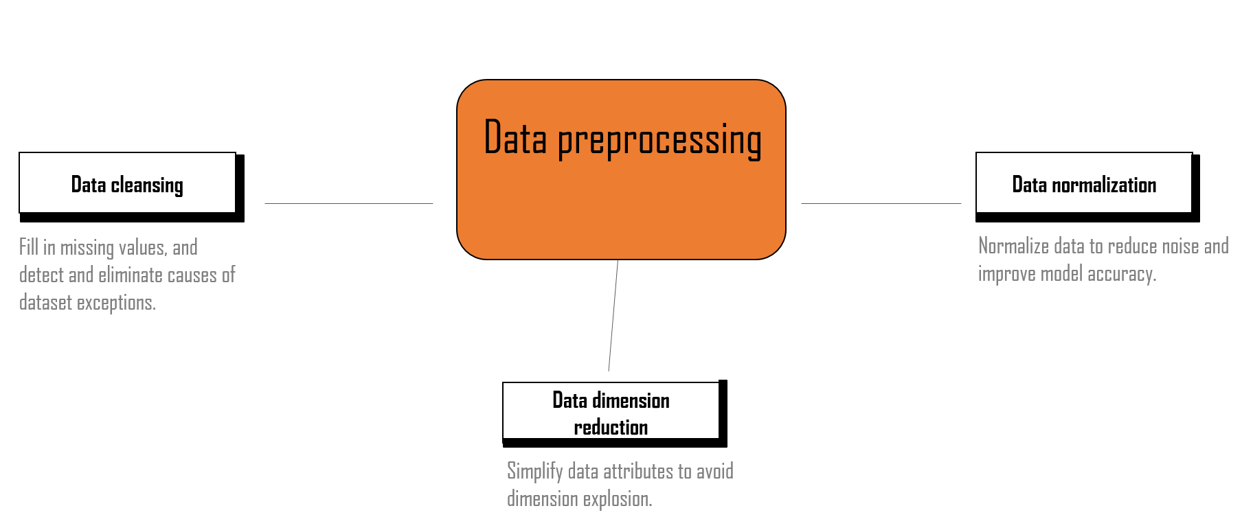
Fill in missing values, and detect and eliminate causes of dataset exceptions.
In most cases, the collected data can be used by algorithms only after being preprocessed. The preprocessing operations include the following:
- Data filtering.
- Processing of lost data.
- Processing of possible exceptions, errors, or abnormal values.
- Combination of data from multiple data sources.
- Data consolidation.
- Generally, real data may have some quality problems.
- Incompleteness: contains missing values or the data that lacks attributes
- Noise: contains incorrect records or exceptions.
- Inconsistency: contains inconsistent records.


- With respect to classification, category data is encoded into a corresponding numerical representation.
- Value data is converted to category data to reduce the value of variables (for age segmentation).
- Other data
- In the text, the word is converted into a word vector through word embedding (generally using the word2vec model, BERT model, etc).
- Process image data (color space, grayscale, geometric change, Haar feature, and image enhancement)
- Feature engineering
- Normalize features to ensure the same value ranges for input variables of the same model.
- Feature expansion: Combine or convert existing variables to generate new features, such as the average.
Generally, a dataset has many features, some of which may be redundant or irrelevant to the value to be predicted.
Feature selection is necessary in the following aspects:
- Simplify models to make them easy for users to interpret
- Reduce the training time
- Avoid dimension explosion
- Improve model generalization and avoid overfitting
Filter methods are independent of the model during feature selection. Procedure of a filter method:
- Traverse all features
- Select the optimal feature subset
- Train models
- Evaluate the performance
By evaluating the correlation between each feature and the target attribute, these methods use a statistical measure to assign a value to each feature. Features are then sorted by score, which is helpful for preserving or eliminating specific features.
Common methods:
- Pearson correlation coefficient
- Chi-square coefficient
- Mutual information
Limitations: The filter method tends to select redundant variables as the relationship between features is not considered.
Wrapper methods use a prediction model to score feature subsets.
Wrapper methods consider feature selection as a search issue for which different combinations are evaluated and compared. A predictive model is used to evaluate a combination of features and assign a score based on model accuracy.
Common methods: Recursive feature elimination (RFE)
Limitations:
- Wrapper methods train a new model for each subset, resulting in a huge number of computations.
- specific type of model
Embedded methods consider feature selection as a part of model construction.
The most common type of embedded feature selection method is the regularization method.
introduce additional constraints into the optimization of a predictive algorithm that bias the model toward lower complexity and reduce the number of features
- Lasso regression
- Ridge regression
Generalization capability: The goal of machine learning is that the model obtained after learning should perform well on new samples, not just on samples used for training. The capability of applying a model to new samples is called generalization or robustness.
Error: difference between the sample result predicted by the model obtained after learning and the actual sample result.
- Training error: error that you get when you run the model on the training data.
- Generalization error: error that you get when you run the model on new samples. Obviously, we prefer a model with a smaller generalization error.
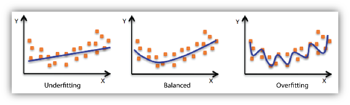
Underfitting: occurs when the model or the algorithm does not fit the data well enough.
Overfitting: occurs when the training error of the model obtained after learning is small but the generalization error is large (poor generalization capability).
Model capacity: model's capability of fitting functions, which is also called model complexity.
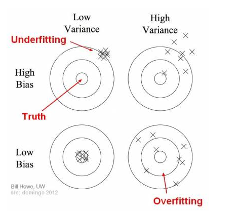
Generally, the prediction error can be divided into two types:
- Variance:
- Offset of the prediction result from the average value
- Error caused by the model's sensitivity to small fluctuations in the training set
- Bias:
- Difference between the expected (or average) prediction value and the correct value we are trying to predict.
Low bias & low variance –> Good model
High bias & high variance –> Poor model
We want a model that can accurately capture the rules in the training data and summarize the invisible data (new data). However, it is usually impossible.
As the model complexity increases,
- the training error decreases.
- the test error decreases to a certain point and then increases in the reverse direction, forming a convex curve
Data Science Modeling: How to Use Linear Regression with Python
The closer the Mean Absolute Error (MAE) is to 0, the better the model can fit the training data.
Mean Square Error (MSE)
The value range of R 2 is (–∞, 1]. A larger value indicates that the model can better fit the training data. TSS indicates the difference between samples. RSS indicates the difference between the predicted value and sample value.
http://qed.econ.queensu.ca/walras/custom/300/351B/notes/reg_08.htm


We have trained a machine learning model to identify whether the object in an image is a cat. Now we use 200 pictures to verify the model performance. Among the 200 images, objects in 170 images are cats, while others are not. The identification result of the model is that objects in 160 images are cats, while others are not.
Precision: P= 140/(140+20) = 87.5%
Recall: R = 140/170 = 82.4%
Accuracy: ACC = (140+10)/(170+30) = 75%
The KNN classification algorithm is a theoretically mature method and one of the simplest machine learning algorithms. According to this method, if the majority of k samples most similar to one sample (nearest neighbors in the eigenspace) belong to a specific category, this sample also belongs to this category.
As the prediction result is determined based on the number and weights of neighbors in the training set, the KNN algorithm has a simple logic
https://www.kdnuggets.com/2016/01/implementing-your-own-knn-using-python.html

- Ensemble learning is a machine learning paradigm in which multiple learners are trained and combined to solve the same problem. When multiple learners are used, the integrated generalization capability can be much stronger than that of a single learner.
- If you ask a complex question to thousands of people at random and then summarize their answers, the summarized answer is better than an expert's answer in most cases. This is the wisdom of the masses.
The chapter describes the basic knowledge of deep learning, including the development history of deep learning, components and types of deep learning neural networks, and common problems in deep learning projects.
As a model based on unsupervised feature learning and feature hierarchy learning, deep learning has great advantages in fields such as computer vision, speech recognition, and natural language processing
Traditional Machine Learning
- Low hardware requirements on the computer: Given the limited computing amount, the computer does not need a GPU for parallel computing generally.
- Applicable to training under a small data amount and whose performance cannot be improved continuously as the data amount increases.
- Level-by-level problem breakdown
- Manual feature selection
- Easy-to-explain features
Deep Learning
Generally, the deep learning architecture is a deep neural network. "Deep" in "deep learning" refers to the number of layers of the neural network.
- Higher hardware requirements on the computer: To execute matrix operations on massive data, the computer needs a GPU to perform parallel computing.
- The performance can be high when highdimensional weight parameters and massive training data are provided.
- E2E learning
- Algorithm-based automatic feature extraction
- Hard-to-explain features
- Currently, the definition of the neural network has not been determined yet. Hecht Nielsen, a neural network researcher in the U.S., defines a neural network as a computer system composed of simple and highly interconnected processing elements
- A neural network can be simply expressed as an information processing system designed to imitate the human brain structure and functions based on its source, features, and explanations.
- Artificial neural network (neural network): Formed by artificial neurons connected to each other, the neural network extracts and simplifies the human brain's microstructure and functions. It is an important approach to simulate human intelligence and reflect several basic features of human brain functions, such as concurrent information processing, learning
- Input vector: 𝑋 = [𝑥0,𝑥1,…,𝑥𝑛]𝑇
- Weight: 𝑊 = [𝜔0,𝜔1,…,𝜔𝑛]𝑇, in which 𝜔0 is the offset.
- Activation function: 𝑂 = 𝑠𝑖𝑔𝑛 𝑛𝑒𝑡 =
- 1,𝑛𝑒𝑡 > 0,
- −1,𝑜𝑡ℎ𝑒𝑟𝑤𝑖𝑠𝑒.
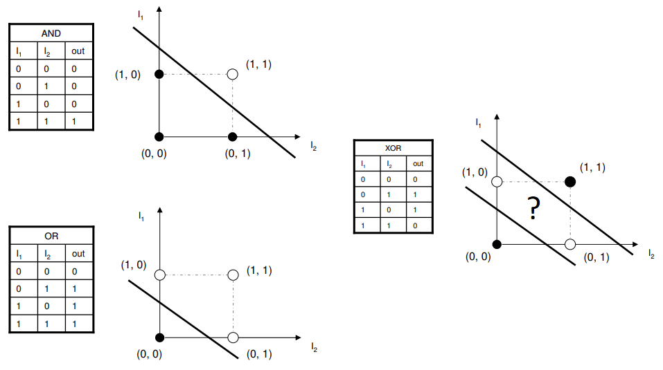
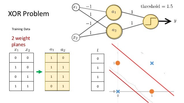
The preceding perceptron is equivalent to a classifier. It uses the high-dimensional 𝑋 vector as the input and performs binary classification on input samples in the high-dimensional space. When 𝑾𝑻𝐗 > 0, O = 1. In this case, the samples are classified into a type. Otherwise, O = −1. In this case, the samples are classified into the other type. The boundary of these two types is 𝑾𝑻𝐗 = 0, which is a high-dimensional hyperplane
A perceptron is essentially a linear model that can only deal with linear classification problems, but cannot process non-linear data.
https://medium.com/@lucaspereira0612/solving-xor-with-a-single-perceptron-34539f395182


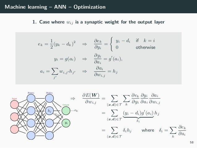
During the training of the deep learning network, target classification errors must be parameterized. A loss function (error function) is used, which reflects the error between the target output and actual output of the perceptron. For a single training sample x, the most common error function is the Quadratic cost function.
The gradient descent method enables the loss function to search along the negative gradient direction and update the parameters iteratively, finally minimizing the loss function.
https://medium.com/machine-learning-for-li/a-walk-through-of-cost-functions-4767dff78f7
Cross entropy error function:
The cross entropy error function depicts the distance between two probability distributions, which is a widely used loss function for classification problems.
Generally, the mean square error function is used to solve the regression problem, while the cross entropy error function is used to solve the classification problem.


In the training sample set 𝐷, each sample is recorded as < 𝑋,𝑡 >, in which 𝑋 is the input vector, 𝑡 the target output, 𝑜 the actual output, and 𝜂 the learning rate.
The gradient descent algorithm of this version is not commonly used because of the convergence process is very slow as all training samples need to be calculated every time the weight is updated.
To address the BGD algorithm defect, a common variant called Incremental Gradient Descent algorithm is used, which is also called the Stochastic Gradient Descent (SGD) algorithm. One implementation is called Online Learning, which updates the gradient based on each sample.
It cannot guarantee to reach the real local minimum as the BGD couold.
To address the defects of the previous two gradient descent algorithms, the Mini-batch Gradient Descent Algorithm (MBGD) was proposed and has been most widely used. A small number of Batch Size (BS) samples are used at a time to calculate ∆𝑤𝑖, and then the weight is updated accordingly.
- Initializes each 𝑤𝑖 to a random value with a smaller absolute value.
- Before the end condition is met:
- Initializes each ∆𝑤𝑖 to zero.
- For the last batch, the training samples are mixed up in a random order.
Signals are propagated in forward direction, and errors are propagated in backward direction. In the training sample set D, each sample is recorded as <X, t>, in which X is the input vector, t the target output, o the actual output, and w the weight coefficient.
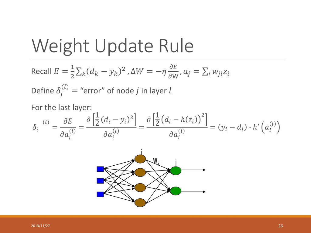
If there are multiple hidden layers, chain rules are used to take a derivative for each layer to obtain the optimized parameters by iteration.
The BP algorithm is used to train the network as follows:
- Takes out the next training sample <X, T>, inputs X to the network, and obtains the actual output o.
- Calculates output layer δ according to the output layer error formula (1).
- Calculates δ of each hidden layer from output to input by iteration according to the hidden layer error propagation formula (2).
- According to the δ of each layer, the weight values of all the layer are updated.
Activation functions are important for the neural network model to learn and understand complex non-linear functions. They allow introduction of non-linear features to the network.
Without activation functions, output signals are only simple linear functions. The complexity of linear functions is limited, and the capability of learning complex function mappings from data is low.

https://deepai.org/machine-learning-glossary-and-terms/softmax-layer
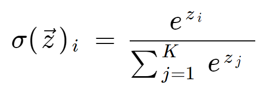
The Softmax function is used to map a K-dimensional vector of arbitrary real values to another K-dimensional vector of real values, where each vector element is in the interval (0, 1). All the elements add up to 1.
The Softmax function is often used as the output layer of a multiclass classification task
Regularization is an important and effective technology to reduce generalization errors in machine learning. It is especially useful for deep learning models that tend to be over-fit due to a large number of parameters. Therefore, researchers have proposed many effective technologies to prevent over-fitting, including
- Adding constraints to parameters, such as 𝐿1 and 𝐿2 norms
- Expanding the training set, such as adding noise and transforming data
- Dropout
- Early stopping
Many regularization methods restrict the learning capability of models by adding a penalty parameter Ω(𝜃) to the objective function 𝐽. Assume that the target function after regularization is 𝐽.
𝐽 (𝜃;𝑋,𝑦) = 𝐽 (𝜃;𝑋,𝑦) + 𝛼Ω(𝜃)Where
𝛼𝜖[0,∞)is a hyperparameter that weights the relative contribution of the norm penalty term Ω and the standard objective function 𝐽(𝑋;𝜃). If 𝛼 is set to 0, no regularization is performed. The penalty in regularization increases with 𝛼.
Add 𝐿1 norm constraint to model parameters, that is 𝐽 𝑤;𝑋,𝑦 = 𝐽 𝑤;𝑋,𝑦 + 𝛼 𝑤 1 If a gradient method is used to resolve the value, the parameter gradient is 𝛻𝐽(𝑤) =∝ 𝑠𝑖𝑔𝑛(𝑤) + 𝛻𝐽(𝑤)
Add norm penalty term 𝐿2 to prevent overfitting. A parameter optimization method can be inferred using an optimization technology (such as a gradient method): 𝑤 = (1 − e𝛼)𝜔 − e𝛻𝐽(𝑤) where e is the learning rate. Compared with a common gradient optimization formula, this formula multiplies the parameter by a reduction factor.
- According to the preceding analysis, 𝐿1 can generate a more sparse model than 𝐿2. When the value of parameter 𝑤 is small, 𝐿1 regularization can directly reduce the parameter value to 0, which can be used for feature selection.
- From the perspective of probability, many norm constraints are equivalent to adding prior probability distribution to parameters. In 𝐿2 regularization, the parameter value complies with the Gaussian distribution rule. In 𝐿1 regularization, the parameter value complies with the Laplace distribution rule
The most effective way to prevent over-fitting is to add a training set. A larger training set has a smaller over-fitting probability. Dataset expansion is a time-saving method, but it varies in different fields.
- A common method in the object recognition field is to rotate or scale images.
- Random noise is added to the input data in speech recognition
- A common practice of natural language processing (NLP) is replacing words with their synonyms
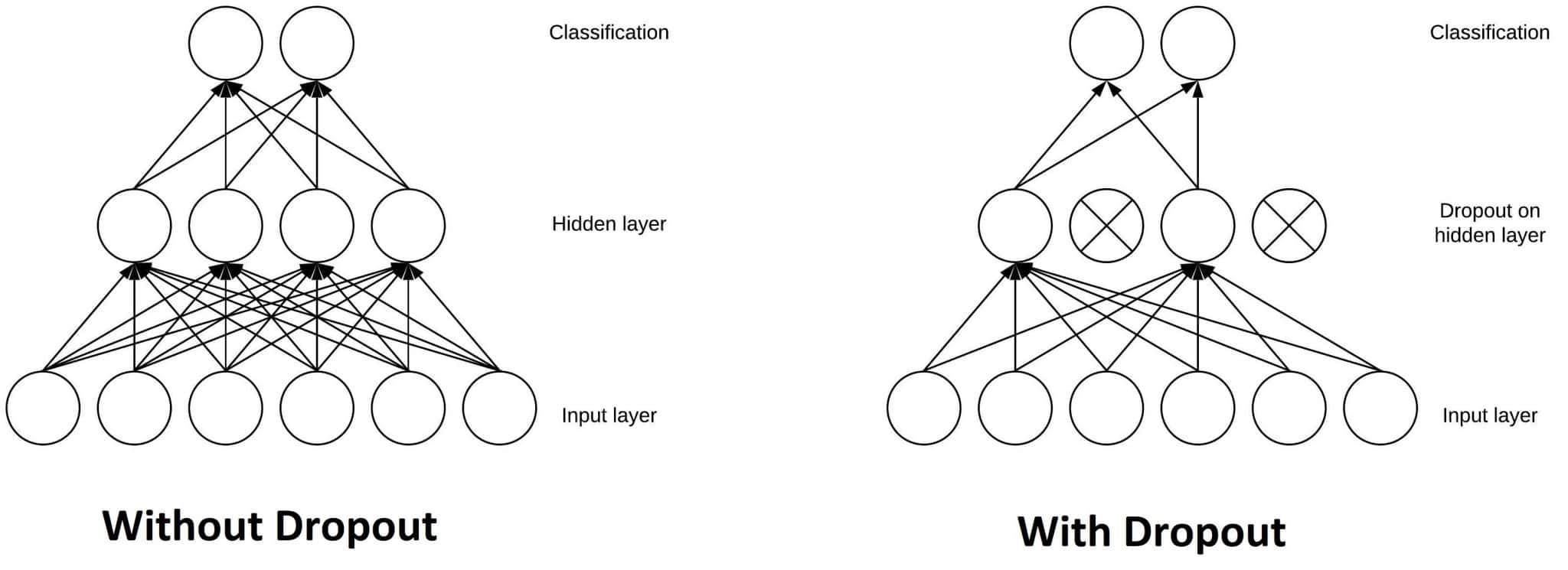
Dropout is a common and simple regularization method, which has been widely used since 2014. Simply put, Dropout randomly discards some inputs during the training process. In this case, the parameters corresponding to the discarded inputs are not updated. As an integration method, Dropout combines all subnetwork results and obtains sub-networks by randomly dropping inputs. See the figures below:
A test on data of the validation set can be inserted during the training. When the data loss of the verification set increases, perform early stopping.

There are various optimized versions of gradient descent algorithms. In objectoriented language implementation, different gradient descent algorithms are often encapsulated into objects called optimizers.
Purposes of the algorithm optimization include but are not limited to:
- Accelerating algorithm convergence
- Preventing or jumping out of local extreme values.
- Simplifying manual parameter setting, especially the learning rate (LR).
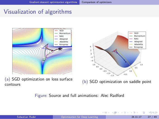
Common optimizers: common GD optimizer, momentum optimizer, Nesterov, AdaGrad, AdaDelta, RMSProp, Adam, AdaMax, and Nadam.
Imagine a small ball rolls down from a random point on the error surface. The introduction of the momentum term is equivalent to giving the small ball inertia.

Advantages:
- Enhances the stability of the gradient correction direction and reduces mutations.
- A small ball with inertia is more likely to roll over some narrow local extrema. Disadvantages: The learning rate 𝜂 and momentum 𝛼 need to be manually set, which often requires more experiments to determine the appropriate value.
The common feature of the random gradient descent algorithm (SGD), small-batch gradient descent algorithm (MBGD), and momentum optimizer is that each parameter is updated with the same LR.
The AdaGrad optimization algorithm shows that the 𝑟 continues increasing while the overall learning rate keeps decreasing as the algorithm iterates. This is because we hope LR to decrease as the number of updates increases. In the initial learning phase, we are far away from the optimal solution to the loss function. As the number of updates increases, we are closer to the optimal solution, and therefore LR can decrease.
- The learning rate is automatically updated. As the number of updates increases, the learning rate decreases.
- The denominator keeps accumulating so that the learning rate will eventually become very small, and the algorithm will become ineffective
The RMSProp optimizer is an improved AdaGrad optimizer. It introduces an attenuation coefficient to ensure a certain attenuation ratio for 𝑟 in each round
The RMSProp optimizer solves the problem that the AdaGrad optimizer ends the optimization process too early. It is suitable for non-stable target handling and has good effects on the RNN.
Adaptive Moment Estimation (Adam): Developed based on AdaGrad and AdaDelta, Adam maintains two additional variables 𝑚𝑡 and 𝑣𝑡 for each variable to be trained:
𝑚𝑡 = 𝛽1𝑚𝑡−1 + (1 − 𝛽1)𝑔𝑡𝑣𝑡 = 𝛽2𝑣𝑡−1 + (1 − 𝛽2)𝑔𝑡^2Where 𝑡 represents the 𝑡-th iteration and 𝑔𝑡 is the calculated gradient. 𝑚𝑡 and 𝑣𝑡 are moving averages of the gradient and square gradient. From the statistical perspective, 𝑚𝑡 and 𝑣𝑡 are estimates of the first moment (the average value) and the second moment (the uncentered variance) of the gradients respectively, which also explains why the method is so named.
If 𝑚𝑡 and 𝑣𝑡 are initialized using the zero vector, 𝑚𝑡 and 𝑣𝑡 are close to 0 during the initial iterations, especially when 𝛽1 and 𝛽2 are close to 1.
n practice, Adam will converge quickly. When convergence saturation is reached, xx can be reduced. After several times of reduction, a satisfying local extremum will be obtained. Other parameters do not need to be adjusted.
[7 Types of Neural Network Activation Functions: How to Choose?]ttps://missinglink.ai/guides/neural-network-concepts/7-types-neural-network-activation-functions-right/#:~:text=Activation%20functions%20are%20mathematical%20equations,relevant%20for%20the%20model's%20prediction.)
- A convolutional neural network (CNN) is a feedforward neural network. Its artificial neurons may respond to surrounding units within the coverage range. CNN excels at image processing. It includes a convolutional layer, a pooling layer, and a fully connected layer.
- n the 1960s, Hubel and Wiesel studied cats' cortex neurons used for local sensitivity and direction selection and found that their unique network structure could simplify feedback neural networks. They then proposed the CNN.
- Now, CNN has become one of the research hotspots in many scientific fields, especially in the pattern classification field. The network is widely used because it can avoid complex pre-processing of images and directly input original images
- Local receptive field: It is generally considered that human perception of the outside world is from local to global. Spatial correlations among local pixels of an image are closer than those among distant pixels. Therefore, each neuron does not need to know the global image. It only needs to know the local image. The local information is combined at a higher level to generate global information.
- Parameter sharing: One or more filters/kernels may be used to scan input images. Parameters carried by the filters are weights. In a layer scanned by filters, each filter uses the same parameters during weighted computation. Weight sharing means that when each filter scans an entire image, parameters of the filter are fixed.

Convolutional Neural Network - CNN -Federal University of Parana
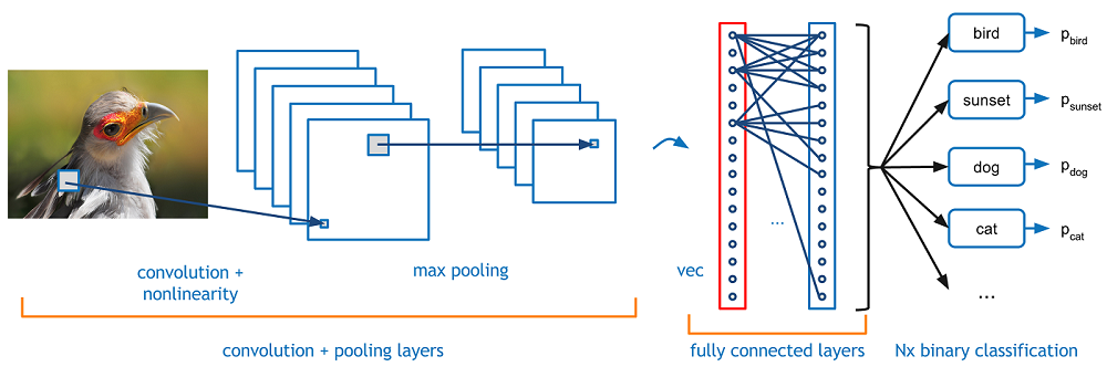
The basic architecture of a CNN is multi-channel convolution consisting of multiple single convolutions. The output of the previous layer (or the original image of the first layer) is used as the input of the current layer. It is then convolved with the filter in the layer and serves as the output of this layer. The convolution kernel of each layer is the weight to be learned. Similar to FCN, after the convolution is complete, the result should be biased and activated through activation functions before being input to the next layer.

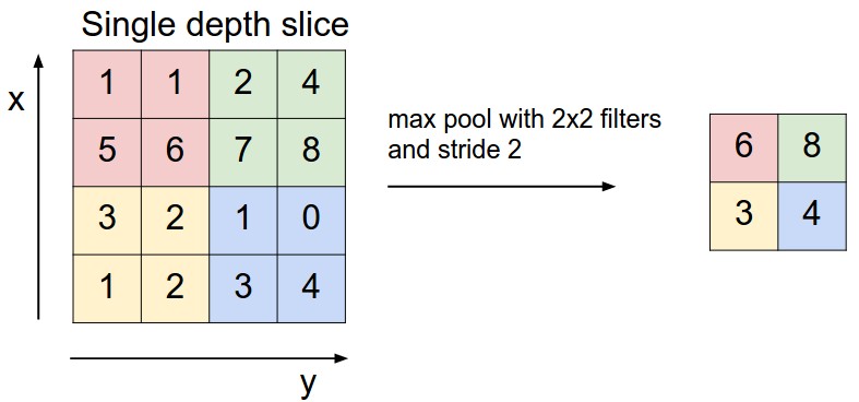
Pooling combines nearby units to reduce the size of the input on the next layer, reducing dimensions. Common pooling includes max pooling and average pooling. When max pooling is used, the maximum value in a small square area is selected as the representative of this area, while the mean value is selected as the representative when average pooling is used. The side of this small area is the pool window size.
The fully connected layer is essentially a classifier. The features extracted on the convolutional layer and pooling layer are straightened and placed at the fully connected layer to output and classify results.
Generally, the Softmax function is used as the activation function of the final fully connected output layer to combine all local features into global features and calculate the score of each type
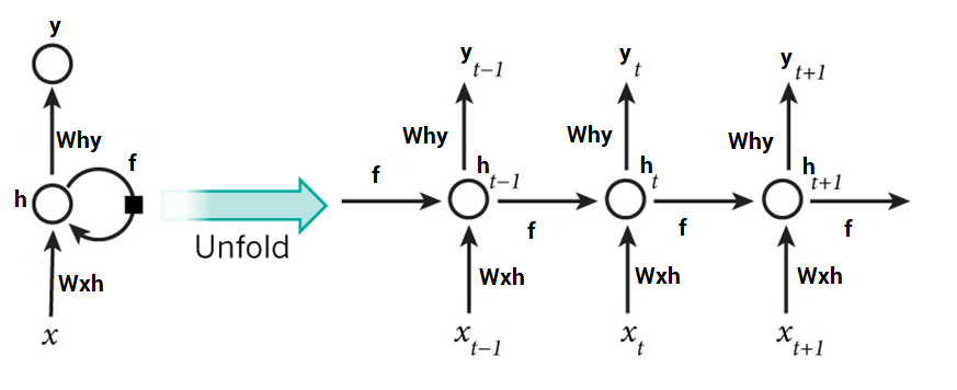
The recurrent neural network (RNN) is a neural network that captures dynamic information in sequential data through periodical connections of hidden layer nodes. It can classify sequential data.
Unlike other forward neural networks, the RNN can keep a context state and even store, learn, and express related information in context windows of any length. Different from traditional neural networks, it is not limited to the space boundary, but also supports time sequences. In other words, there is a side between the hidden layer of the current moment and the hidden layer of the next moment.
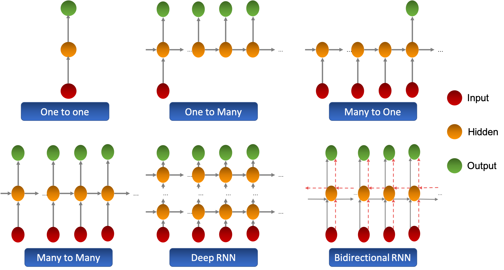
The RNN is widely used in scenarios related to sequences, such as videos consisting of image frames, audio consisting of clips, and sentences consisting of words.
- Traditional backpropagation is the extension on the time sequence.
- There are two sources of errors in the sequence at time of memory unit: first is from the hidden layer output error at t time sequence; the second is the error from the memory cell at the next time sequence t + 1.
- The longer the time sequence, the more likely the loss of the last time sequence to the gradient of w in the first time sequence causes the vanishing gradient or exploding gradient problem.
- The total gradient of weight w is the accumulation of the gradient of the weight at all time sequence.
- Updating weights using the SGD algorithm
Three steps of BPTT:
- Computing the output value of each neuron through forward propagation.
- Computing the error value of each neuron through backpropagation 𝛿𝑗.
- Computing the gradient of each weight.
- Despite that the standard RNN structure solves the problem of information memory, the information attenuates during long-term memory.
- Information needs to be saved long time in many tasks. For example, a hint at the beginning of a speculative fiction may not be answered until the end
- The RNN may not be able to save information for long due to the limited memory unit capacity.
- We expect that memory units can remember key information.
https://mreza-rezaei.github.io/Generative-Nets/
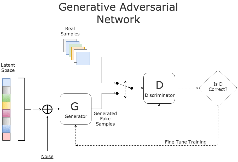
- Generative Adversarial Network is a framework that trains generator G and discriminator D through the adversarial process. Through the adversarial process, the discriminator can tell whether the sample from the generator is fake or real. GAN adopts a mature BP algorithm.
- Generator G: The input is noise z, which complies with manually selected prior probability distribution, such as even distribution and Gaussian distribution. The generator adopts the network structure of the multilayer perceptron (MLP), uses maximum likelihood estimation (MLE) parameters to represent the derivable mapping G(z), and maps the input space to the sample space.
- Discriminator D: The input is the real sample x and the fake sample G(z), which are tagged as real and fake respectively. The network of the discriminator can use the MLP carrying parameters. The output is the probability D(G(z)) that determines whether the sample is a real or fake sample.
- GAN can be applied to scenarios such as image generation, text generation, speech enhancement, image super-resolution.
- In the early training stage, when the outcome of G is very poor, D determines that the generated sample is fake with high confidence, because the sample is obviously different from training data.
- Problem description: In the dataset consisting of various task categories, the number of samples varies greatly from one category to another. One or more categories in the predicted categories contain very few samples.
- For example, in an image recognition experiment, more than 2,000 categories among a total of 4251 training images contain just one image each. Some of the others have 2-5 images.
- Due to the unbalanced number of samples, we cannot get the optimal real-time result because model/algorithm never examines categories with very few samples adequately
- Since few observation objects may not be representative for a class, we may fail to obtain adequate samples for verification and test
- Vanishing gradient: As network layers increase, the derivative value of backpropagation decreases, which causes a vanishing gradient problem.
- Exploding gradient: As network layers increase, the derivative value of backpropagation increases, which causes an exploding gradient problem.
- Overfitting
- the model performs well in the training set, but badly in the test set.
- Root cause: There are too many feature dimensions, model assumptions, and parameters, too much noise, but very few training data. As a result, the fitting function perfectly predicts the training set, while the prediction result of the test set of new data is poor. Training data is over-fitted without considering generalization capabilities.
- Solution: For example, data augmentation, regularization, early stopping, and dropout
A deep learning framework is an interface, library or a tool which allows us to build deep learning models more easily and quickly, without getting into the details of underlying algorithms. A deep learning framework can be regarded as a set of building blocks. Each component in the building blocks is a model or algorithm. Therefore, developers can use components to assemble models that meet requirements, and do not need to start from scratch.
The emergence of deep learning frameworks lowers the requirements for developers. Developers no longer need to compile code starting from complex neural networks and back-propagation algorithms. Instead, they can use existing models to configure parameters as required, where the model parameters are automatically trained. Moreover, they can add self-defined network layers to the existing models, or select required classifiers and optimization algorithms directly by invoking existing code.
PyTorch is a Python-based machine learning computing framework developed by Facebook. It is developed based on Torch, a scientific computing framework supported by a large number of machine learning algorithms. Torch is a tensor operation library similar to NumPy, featured by high flexibility, but is less popular because it uses the programming language Lua.
- Python first: PyTorch does not simply bind Python to a C++ framework. PyTorch directly supports Python access at a fine grain. Developers can use PyTorch as easily as using NumPy or SciPy. This not only lowers the threshold for understanding Python, but also ensures that the code is basically consistent with the native Python implementation.
- Dynamic neural network: Many mainstream frameworks such as TensorFlow 1.x do not support this feature. To run TensorFlow 1.x, developers must create static computational graphs in advance, and run the feed and run commands to repeatedly execute the created graphs. In contrast, PyTorch with this feature is free from such complexity, and PyTorch programs can dynamically build/adjust computational graphs during execution.
- Easy to debug: PyTorch can generate dynamic graphs during execution. Developers can stop an interpreter in a debugger and view output of a specific node.
- PyTorch provides tensors that support CPUs and GPUs, greatly accelerating computing
TensorFlow is Google's second-generation open-source software library for digital computing. The TensorFlow computing framework supports various deep learning algorithms and multiple computing platforms, ensuring high system stability.
- Multi-lingual
- Multi-platform
- Distributed
- scalability
- GPU
- Powerful computing
- TensorFlow can run on different computers: From smartphones to computer clusters, to generate desired training models
- Currently, supported native distributed deep learning frameworks include only TensorFlow, CNTK, Deeplearning4J, and MXNet
- When a single GPU is used, most deep learning frameworks rely on cuDNN, and therefore support almost the same training speed, provided that the hardware computing capabilities or allocated memories slightly differ. However, for largescale deep learning, massive data makes it difficult for the single GPU to complete training in a limited time. To handle such cases, TensorFlow enables distributed training. TensorFlow is considered as one of the best libraries for neural networks, and can reduce difficulty in deep learning development. In addition, as it is open-source, it can be conveniently maintained and updated, thus the efficiency of development can be improved.
Keras, ranking third in the number of stars on GitHub, is packaged into an advanced API of TensorFlow 2.0, which makes TensorFlow 2.x more flexible, and easier to debug.
Disadvantages of TensorFlow 1.0:
- After a tensor is created in TensorFlow 1.0, the result cannot be returned directly. To obtain the result, the session mechanism needs to be created, which includes the concept of graph, and code cannot run without session.run. This style is more like the hardware programming language VHDL.
- Compared with some simple frameworks such as PyTorch, TensorFlow 1.0 adds the session and graph concepts, which are inconvenient for users.
- It is complex to debug TensorFlow 1.0, and its APIs are disordered, making it difficult for beginners. Learners will come across many difficulties in using TensorFlow 1.0 even after gaining the basic knowledge.
Features of TensorFlow 2.x:
- Easy to use: The graph and session mechanisms are removed. What you see is what you get, just like Python and PyTorch.
- The core function of TensorFlow 2.x is the dynamic graph mechanism called eager execution. It allows users to compile and debug models like normal programs, making TensorFlow easier to learn and use.
- Multiple platforms and languages are supported
- Deprecated APIs are deleted and duplicate APIs are reduced to avoid confusion
- Compatibility and continuity: TensorFlow 2.x provides a module enabling compatibility with TensorFlow 1.x.
- The tf.contrib module is removed. Maintained modules are moved to separate repositories
Tensors are the most basic data structures in TensorFlow. All data is encapsulated in tensors.

In TensorFlow, tensors are classified into:
- Constant tensors
- Variable tensors
The following describes common APIs in TensorFlow by focusing on code. The main content is as follows:
- Methods for creating constants and variables
- Tensor slicing and indexing
- Dimension changes of tensors
- Arithmetic operations on tensors
- Tensor concatenation and splitting
- Tensor sorting
Static graph: TensorFlow 1.x using static graphs (graph mode) separates computation definition and execution by using computational graphs. This is a declarative programming model. In graph mode, developers need to build a computational graph, start a session, and then input data to obtain an execution result.
Static graphs are advantageous in distributed training, performance optimization, and deployment, but inconvenient for debugging. Executing a static graph is similar to invoking a compiled C language program, and internal debugging cannot be performed in this case. Therefore, eager execution based on dynamic computational graphs emerges.
Eager execution is a command-based programming method, which is the same as native Python. A result is returned immediately after an operation is performed
Eager execution is enabled in TensorFlow 2.x by default. Eager execution is intuitive and flexible for users (easier and faster to run a one-time operation), but may compromise performance and deployability.
To achieve optimal performance and make a model deployable anywhere, you can run @tf.function to add a decorator to build a graph from a program, making Python code more efficient.
tf.function can build a TensorFlow operation in the function into a graph. In this way, this function can be executed in graph mode. Such practice can be considered as encapsulating the function as a TensorFlow operation of a graph.

tf: Functions in the tf module are used to perform common arithmetic operations, such astf.abs(calculating an absolute value),tf.add(adding elements one by one), andtf.concat(concatenating tensors). Most operations in this module can be performed by NumPy.tf.errors: error type module of TensorFlowtf.data: implements operations on datasets; Input pipes created by tf.data are used to read training data. In addition, data can be easily input from memories (such as NumPy).tf.distributions: implements various statistical distributions; The functions in this module are used to implement various statistical distributions, such as Bernoulli distribution, uniform distribution, and Gaussian distribution.tf.io.gfile: implements operations on files. Functions in this module can be used to perform file I/O operations, copy files, and rename files.tf.image: implements operations on images; Functions in this module include image processing functions. This module is similar to OpenCV, and provides functions related to image luminance, saturation, phase inversion, cropping, resizing, image format conversion (RGB to HSV, YUV, YIQ, or gray), rotation, and sobel edge detection. This module is equivalent to a small image processing package of OpenCV.tf.keras: a Python API for invoking Keras tools. This is a large module that enables various network operations
TensorFlow 2.x recommends Keras for network building. Common neural networks are included in Keras.layers. Keras is a high-level API used to build and train deep learning models. It can be used for rapid prototype design, advanced research, and production. It has the following three advantages:
- Keras provides simple and consistent GUIs optimized for common cases. It provides practical and clear feedback on user errors.
- You can build Keras models by connecting configurable building blocks together, with little restriction.
- You can customize building blocks to express new research ideas, create layers and loss functions, and develop advanced models.
The following describes common methods and interfaces of tf.keras by focusing on code. The main content is as follows:
- Dataset processing: datasets and preprocessing
- Neural network model creation: Sequential, Model, Layers...
- Network compilation: compile, Losses, Metrics, and Optimizers
- Network training and evaluation: fit, fit_generator, and evaluate
Environment setup in Windows 10:
pip software built in Anaconda 3 (adapting to Python 3)- TensorFlow installation
- Open Anaconda Prompt and run the
pipcommand to install TensorFlow- Run
pip install TensorFlowin the command line interface Linux: The simplest way for installing TensorFlow is to run the pip command:pip install TensorFlow==2.1.0
- Data preparation
- Network construction
- Model training and verification
- Model saving
- Model restoration and invoking
Handwritten digit recognition is a common image recognition task where computers recognize text in handwriting images. Different from printed fonts, handwriting of different people has different sizes and styles, making it difficult for computers to recognize handwriting. This project applies deep learning and TensorFlow tools to train and build models based on the MNIST handwriting dataset.
- Download the MNIST datasets from http://yann.lecun.com/exdb/mnist/.
- Training set: 60,000 handwriting images and corresponding labels
- Test set: 10,000 handwriting images and corresponding labels
The softmax function is also called normalized exponential function. It is a derivative of the binary classification function sigmoid in terms of multi-class classification.
- The process of model establishment is the core process of network structure definition.
- The network operation process defines how model output is calculated based on input.
- Matrix multiplication and vector addition are used to express the calculation process of softmax
## import tensorflow
import tensorflow as tf
##define input variables with operator symbol variables.
‘’’ we use a variable to feed data into the graph through the placeholders X. Each input image is flattened into a 784-dimensional vector. In this case, the shape of the tensor is [None, 784], None indicates can be of any length. ’’’
X = tf.placeholder(tf.float32,[None,784])
‘’’ The variable that can be modified is used to indicate the weight w and bias b. The initial values are set to 0. ’’’
w = tf.Variable(tf.zeros([784,10]))
b = tf.Variable(tf.zeros([10]))
‘’’ If tf.matmul(x, w) is used to indicate that x is multiplied by w, the Soft regression equation is y = softmax(wx+b)'‘’
y = tf.nn.softmax(tf.matmul(x,w)+b) In machine learning/deep learning, an indicator needs to be defined to indicate whether a model is proper. This indicator is called cost or loss, and is minimized as far as possible. In this project, the cross entropy loss function is used.
A loss function is constructed for an original model needs to be optimized by using an optimization algorithm, to find optimal parameters and further minimize a value of the loss function. Among optimization algorithms for solving machine learning parameters, the gradient descent-based optimization algorithm (Gradient Descent) is usually used.
model.compile(optimizer=tf.train.AdamOptimizer(), loss=tf.keras.losses.categorical_crossentropy, metrics=[tf.keras.metrics.categorical_accuracy])- All training data is trained through batch iteration or full iteration. In the experiment, all data is trained five times.
- In TensorFlow,
model.fitis used for training, where epoch indicates the number of training iterations.
You can test the model using the test set, compare predicted results with actual ones, and find correctly predicted labels, to calculate the accuracy of the test set.
[loss accuracy]
This chapter introduces the structure, design concept, and features of MindSpore based on the issues and difficulties facing by the AI computing framework, and describes the development and application process in MindSpore.

Ultra-large models realize efficient distributed training: As NLP-domain models swell, the memory overhead for training ultra-large models such as Bert (340M)/GPT-2(1542M) has exceeded the capacity of a single card. Therefore, the models need to be split into multiple cards before execution. Manual model parallelism is used currently. Model segmentation needs to be designed and the cluster topology needs to be understood. The development is extremely challenging. The performance is lackluster and can be hardly optimized.
Automatic graph segmentation: It can segment the entire graph based on the input and output data dimensions of the operator, and integrate the data and model parallelism. Cluster topology awareness scheduling: It can perceive the cluster topology, schedule subgraphs automatically, and minimize the communication overhead
Challenges for model execution with supreme chip computing power: Memory wall, high interaction overhead, and data supply difficulty. Partial operations are performed on the host, while the others are performed on the device. The interaction overhead is much greater than the execution overhead, resulting in the low accelerator usage
Challenges for model execution with supreme chip computing power: Memory wall, high interaction overhead, and data supply difficulty. Partial operations are performed on the host, while the others are performed on the device. The interaction overhead is much greater than the execution overhead, resulting in the low accelerator usage.
Chip-oriented deep graph optimization reduces the synchronization waiting time and maximizes the parallelism of data, computing, and communication. Data pre-processing and computation are integrated into the Ascend chip.
Challenges for distributed gradient aggregation with supreme chip computing power: the synchronization overhead of central control and the communication overhead of frequent synchronization of ResNet50 under the single iteration of 20 ms; the traditional method can only complete All Reduce after three times of synchronization, while the data-driven method can autonomously perform All Reduce without causing control overhead
The optimization of the adaptive graph segmentation driven by gradient data can realize decentralized All Reduce and synchronize gradient aggregation, boosting computing and communication efficiency
The diversity of hardware architectures leads to fullscenario deployment differences and performance uncertainties. The separation of training and inference leads to isolation of models
Unified model IR delivers a consistent deployment experience. The graph optimization technology featuring software and hardware collaboration bridges different scenarios. Device-cloud Synergy Federal Meta Learning breaks the devicecloud boundary and updates the multi-device collaboration model in real time
Install: https://www.mindspore.cn/install/en
In MindSpore, data is stored in tensors. Common tensor operations:
asnumpy()size()dim()dtype()set_dtype()tensor_add(other: Tensor)tensor_mul(other: Tensor)shape()__Str__# (conversion into strings)
Common operations in MindSpore:
array: Array-related operatorsmath: Math-related operatorsnn: Network operatorscontrol: Control operatorsrandom: Random operators
A cell defines the basic module for calculation. The objects of the cell can be directly executed.
__init__: It initializes and verifies modules such as parameters, cells, and primitives.Construct: It defines the execution process. In graph mode, a graph is compiled for execution and is subject to specific syntax restrictionsbprop(optional): It is the reverse direction of customized modules. If this function is undefined, automatic differential is used to calculate the reverse of the construct part
Cells predefined in MindSpore mainly include: common loss (Softmax Cross Entropy With Logits and MSELoss), common optimizers (Momentum, SGD, and Adam), and common network packaging functions, such as TrainOneStepCell network gradient calculation and update, and WithGradCell gradient calculation
MindSporeIR is a compact, efficient, and flexible graph-based functional IR that can represent functional semantics such as free variables, high-order functions, and recursion. It is a program carrier in the process of AD and compilation optimization.
Each graph represents a function definition graph and consists of ParameterNode, ValueNode, and ComplexNode (CNode).
The figure shows the def-use relationship.
Let’s take the recognition of MNIST handwritten digits as an example to demonstrate the modeling process in MindSpore.
Data
- Data loading
- Data enhancement
Network 3. Network definition 4. Weight initialization 5. Network execution
Model 6. Loss function 7. Optimizer 8. Training iteration 9. Model evaluation
Application 10. Model saving 11. Load prediction 12. Fine tuning
Ascend is a chip where Atlas is the computing platform
AI chips, also known as AI accelerators, are function modules that process massive computing tasks in AI applications.
AI Chips can be divided into four types by technical architecture:
- A central processing unit (CPU): a super-large-scale integrated circuit, which is the computing core and control unit of a computer. It can interpret computer instructions and process computer software data.
- A graphics processing unit (GPU): a display core, visual processor, and display chip. It is a microprocessor that processes images on personal computers, workstations, game consoles, and mobile devices, such as tablet computers and smart phones.
- An application specific integrated circuit (ASIC): an integrated circuit designed for a specific purpose
- A field programmable gate array (FPGA): designed to implement functions of a semicustomized chip. The hardware structure can be flexibly configured and changed in real time based on requirements.
AI chips can be divided into training and inference by business application:
- In the training phase, a complex deep neural network model needs to be trained through a large number of data inputs or an unsupervised learning method such as enhanced learning. The training process requires massive training data and a complex deep neural network structure. The huge computing amount requires ultra-high performance including computing power, precision, and scalability of processors. Nvidia GPU cluster and Google TPUs are commonly used in AI training.
- Inferences are made using trained models and new data. For example, a video surveillance device uses the background deep neural network model to recognize a captured face. Although the calculation amount of the inference is much less than that of training, a large number of matrix operations are involved. GPU, FPGA and ASIC are also used in the inference process.
- The computer performance has been steadily improved based on the Moore's Law
- The CPU cores added for performance enhancement also increase power consumption and cost
- Extra instructions have been introduced and the architecture has been modified to improve AI performance.
- Despite that boosting the processor frequency can elevate the performance, the high frequency will cause huge power consumption and overheating of the chip as the frequency reaches the ceiling.
- GPU performs remarkably in matrix computing and parallel computing and plays a key role in heterogeneous computing. It was first introduced to the AI field as an acceleration chip for deep learning. Currently, the GPU ecosystem has matured.
- Using the GPU architecture, NVIDIA focuses on the following two aspects of deep learning:
- Diversifying the ecosystem: It has launched the cuDNN optimization library for neural networks to improve usability and optimize the GPU underlying architecture.
- Improving customization: It supports various data types, including int8 in addition to float32; introduces modules dedicated for deep learning.
- The existing problems include high costs and latency and low energy efficiency
Massive systolic arrays and large-capacity on-chip storage are adopted to accelerate the most common convolution operations in deep neural networks.
- Using the HDL programmable mode, FPGAs are highly flexible, reconfigurable and reprogrammable, and customizable.
- the design and tapeout processes are decoupled. The development period is long, generally half a year. The entry barrier is high
- GPUs are designed for massive data of the same type independent from each other and pure computing environments that do not need to be interrupted.
- CPUs need to process different data types in a universal manner, perform logic judgment, and introduce massive branch jumps and interrupted processing
Neural-network processing unit (NPU): uses a deep learning instruction set to process a large number of human neurons and synapses simulated at the circuit layer. One instruction is used to process a group of neurons.
Typical NPUs: Huawei Ascend AI chips, Cambricon chips, and IBM TrueNorth
- controrl cpu
- ai computing engine including ai core and ai cpu
- multi lyaer system on chip
computing unit
- cube, vector and scalar units corrersond to matrix vector and scalar computing modes respectively
- cube: The matrix computing unit and accumulator are used to perform matrix-related operations. Completes a matrix (4096) of 16x16 multiplied by 16x16 for FP16, or a matrix (8192) of 16x32 multiplied by 32x16 for the INT8 input in a shot.
- Vector computing unit: implements computing between vectors and scalars or between vectors. This function covers various basic computing types and many customized computing types, including computing of data types such as FP16, FP32, INT32, and INT8.
- Scalar computing unit: Equivalent to a micro CPU, the scalar unit controls the running of the entire AI core. It implements loop control and branch judgment for the entire program, and provides the computing of data addresses and related parameters for cubes or vectors as well as basic arithmetic operations
Storage System
- The storage system of the AI core is composed of the storage unit and corresponding data channel.
- the storage unit consists of the storage control unit, buffer, and registers:
- Storage control unit: The cache at a lower level than the AI core can be directly accessed through the bus interface. The memory can also be directly accessed through the DDR or HBM. A storage conversion unit is set as a transmission controller of the internal data channel of the AI core to implement read/write management of internal data of the AI core between different buffers. It also completes a series of format conversion operations, such as zero padding, Img2Col, transposing, and decompression.
- input buffer: The buffer temporarily stores the data that needs to be frequently used so the data does not need to be read from the AI core through the bus interface each time. This mode reduces the frequency of data access on the bus and the risk of bus congestion, thereby reducing power consumption and improving performance.
- Output buffer: The buffer stores the intermediate results of computing at each layer in the neural network, so that the data can be easily obtained for next-layer computing. Reading data through the bus involves low bandwidth and long latency, whereas using the output buffer greatly improves the computing efficiency
Data channel: path for data flowing in the AI core during execution of computing tasks. A data channel of the Da Vinci architecture is characterized by multiple-input single-output. Considering various types and a large quantity of input data in the computing process on the neural network, parallel inputs can improve data inflow efficiency. On the contrary, only an output feature matrix is generated after multiple types of input data are processed. The data channel with a single output of data reduces the use of chip hardware resources.
The control unit consists of the system control module, instruction cache, scalar instruction processing queue, instruction transmitting module, matrix operation queue, vector operation queue, storage conversion queue, and event synchronization module.
This section describes the software architecture of Ascend chips, including the logic architecture and neural network software flow of Ascend AI processors.
L3 application enabling layer: It is an application-level encapsulation layer that provides different processing algorithms for specific application fields. L3 provides various fields with computing and processing engines. It can directly use the framework scheduling capability provided by L2 to generate corresponding NNs and implement specific engine functions.
L2 execution framework layer: encapsulates the framework calling capability and offline model generation capability. After the application algorithm is developed and encapsulated into an engine at L3, L2 calls the appropriate deep learning framework, such as Caffe or TensorFlow, based on the features of the algorithm to obtain the neural network of the corresponding function, and generates an offline model through the framework manager. After L2 converts the original neural network model into an offline model that can be executed on Ascend AI chips, the offline model executor (OME) transfers the offline model to Layer 1 for task allocation.
L1 chip enabling layer: bridges the offline model to Ascend AI chips. L1 accelerates the offline model for different computing tasks via libraries.
L0 computing resource layer: provides computing resources and executes specific computingtasks. It is the hardware computing basis of the Ascend AI chip.
Camera data collection and processing
- Compressed video streams are transmitted from the camera to the DDR memory through PCIe
- DVPP reads the compressed video streams into the cache.
- After preprocessing, DVPP writes decompressed frames into the DDR memory.
- Data inference
- The task scheduler (TS) sends an instruction to the DMA engine to pre-load the AI resources from the DDR to the on-chip buffer.
- The TS configures the AI core to execute tasks.
- The AI core reads the feature map and weight, and writes the result to the DDR or on-chip buffer
Facial recognition result output:
- After processing, the AI core sends the signals to the TS, which checks the result.
- When the last AI task is complete, the TS reports the result to the host.
Huawei HiAI is an open artificial intelligence (AI) capability platform for smart devices, which adopts a "chip-device-cloud" architecture, opening up chip, app, and service capabilities for a fully intelligent ecosystem. This assists developers in delivering a better smart app experience for users by fully leveraging Huawei's powerful AI processing capabilities.
- High thresholds
- Low efficiency
- Diverse requests
- Slow iteration
HiAI Foundation APIs constitute an AI computing library of a mobile computing platform, enabling developers to efficiently compile AI apps that can run on mobile devices.
Support the largest number of operators (300+) in the industry and more frameworks, greatly improving flexibility and compatibility.
HiAI Engine opens app capabilities and integrates multiple AI capabilities into apps, making apps smarter and more powerful.
Provide handwriting recognition and dynamic gesture recognition capabilities, with 40+ underlying APIs.
HiAI Service enables developers to reuse services on multiple devices, such as mobile phones, tablets, and large screens, with only one service access, efficiently implementing distribution.
On completion of this course, you will be able to:
- Know the HUAWEI CLOUD enterprise intelligence (EI) ecosystem and services.
- Know the Huawei ModelArts platform and how to perform operations on the platform
HUAWEI CLOUD EI is a driving force for enterprises' intelligent transformation. Relying on AI and big data technologies, HUAWEI CLOUD EI provides an open, trustworthy, and intelligent platform through cloud services (in mode such as public cloud or dedicated cloud).
EI Intelligent Twins
The EI Intelligent Twins integrates AI technologies into application scenarios of various industries and fully utilizes advantages of AI technologies to improve efficiency and experience.
Traffic Intelligent Twins (TrafficGo)
The Traffic Intelligent Twins (TrafficGo) enables 24/7 and all-area traffic condition monitoring, traffic incident detection, realtime traffic signal scheduling, traffic situation large-screen display, and key vehicle management, delivering an efficient, environment-friendly, and safe travel experience.
Industrial Intelligent Twins
The Industrial Intelligent Twins uses big data and AI technologies to provide a full series of services covering design, production, logistics, sales, and service. It helps enterprises gain a leading position
Campus Intelligent Twins
The Campus Intelligent Twins manages and monitors industrial, residential, and commercial campuses. It adopts AI technologies such as video analytics and data mining to make our work and life more convenient and efficient.
HiLens
https://support.huaweicloud.com/intl/en-us/productdesc-hilens/hilens_01_0001.html
Huawei HiLens consists of computing devices and a cloud-based development platform, and provides a development framework, a development environment, and a management platform to help users develop multimodal AI applications and deliver them to devices, to implement intelligent solutions in multiple scenarios.

GES
GES facilitates query and analysis of graph-structure data based on various relationships. It uses the high performance graph engine EYWA as its kernel, and is granted many independent intellectual property rights. GES plays an important role in scenarios such as social apps, enterprise relationship analysis applications, logistics distribution, shuttle bus route planning, enterprise knowledge graph, and risk control.
Conversational Bot Service (CBS)
- Question-Answering bot (QABot
- Task-oriented conversational bot (TaskBot)
- Speech analytics
- CBS customization
EI Experience Center
The EI Experience Center is an AI experience window built by Huawei, dedicated to lowering the threshold for using AI and making AI ubiquitous.
ModelArts is a one-stop development platform for AI developers. With data preprocessing, semi-automatic data labeling, large-scale distributed training, automatic modeling, and on-demand model deployment on devices, edges, and clouds, ModelArts helps AI developers build models quickly and manage the AI development lifecycle. https://www.huaweicloud.com/en-us/product/modelarts.html