Francesco Pisu, Hicham Lafhouli
- Regression Analysis for Used Car Price Prediction
- 2. Notebook structure
- 3. Methodology
- 4. Comparing regression models
- 5. Experimental Results
- 6. Conclusions
This project aims to solve the problem of predicting the price of a used car, using Sklearn's supervised machine learning techniques integrated with Spark-Sklearn library. It is clearly a regression problem and predictions are carried out on dataset of used car sales in the american car market. Several regression tecniques have been studied, including Linear Regression, Decision Trees and Random forests of decision trees. Their performances were compared in order to determine which one works best with out dataset.
This project is available as a Google Colaboratory Notebook at the following link.
Most of the project has been developed using Python as the programming language of choice and the following libraries:
- Scikit-Learn, regression models and cross validation techniques.
- Spark-Sklearn, parallelization of the hyperparameter tuning process.
- Pandas, data analysis purposes.
- ELK Stack, data analysis too.
- Rfpimp, feature importances in random forests.
Last but not least, Google Colaboratory was the computing platform of choice for training and testing our models.
Used car price prediction problem has a certain value because different studies show that the market of used cars is destined to a continuous growth in the short term. In fact, leasing cars is now a common practice through which it is possible to get get hold of a car by paying a fixed sum for an agreed number of months rather than buying it in its entirety. Once leasing period is over, it is possible to buy the car by paying the residual value, i.e. at the expected resale price. It is therefore in the interest of vendors to be able to predict this value with a certain degree of accuracy, since if this value is initially underestimated, the installment will be higher for the customer which will most likely opt for another dealership. It is therefore clear that the price prediction of used cars has a high commercial value, especially in developed countries where the economy of leasing has a certain volume.
This problem, however, is not easy to solve as the car's value depends on many factor including year of registration, manufacturer, model, mileage, horsepower, origin and several other specific informations such as type of fuel and braking sysrem, condition of bodywork and interiors, interior materials (plastics of leather), safery index, type of change (manual, assisted, automatic, semi-automatic), number of doors, number of previous owners, if it was previously owned by a private individual or by a company and the prestige of the manufacturer.
Unfortunately, only a small part of this information is available and therefore it is very important to relate the results obtained in terms of accuracy to the features available for the analysis. Moreover, not all the previously listed features have the same importance, some are more so than others and therefore is essential to identify the most important ones, on which to perform the analysis.
Since some attributes of the dataset aren't relevant to our analysis, they have been discarded; so, as mentioned above, this fact must be taken into account when conclusions on the accuracy are drawn.
The python notebook is structured as follows:
Notebook structure
Used_car_price_prediction:
│   installing libraries
│   imports
│   read csv file
│
└─── Price attribute analysis
│     relationship with numerical features
│     relationship with categorical features
│     feature importance related to price
│     correlation matrices (price and general)
│     scatterplots
|
└─── Preprocessing
│     outliers management
│         │     bivariate analysis
│         │     removing outliers by model
│         │     read new csv file (cleaned_cars)
│         │     final outliers removal
│         --------------------------------------
│     towards normal distribution of prices
│     label encoding
│     train/test split
|
└─── Training and evaluating models
│     function definitions
│     linear regressor
│     decision tree regressor
│         |     complexity curve
│         ----------------------
│     random forest regressor
│         |     complexity curve
│         ----------------------
|
└─── Cross validation
│     linear regression
│     decision tree regression
│     random forest regression
|
└─── Predictions on final model and conclusions
|     feature importance
This chapter provides an in-depth description of the followed methodology for solving the problem discussed above, with particular emphasis on the first phase concerning the dataset analysis carried out with ELK stack and the consequent preprocessing of data, followed by the definition, training and evaluation of the chosen regression models, highlighting the importance of integrating these techniques with Spark to parallelize the process of hyperparameter tuning of decision models.
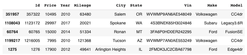
The dataset on which the regression analysis was performed consists of approximately 1.2 milion records of used car sales in the american market from 1997 to 2018, acquired via scraping on TrueCar.com car sales portal.
Each record has the following features: Id, price, year, mileage, city, state, license plate, manufacturer and model.
ELK Stack is a set of Open Source products designed by Elastic for analizing and visualizing data of any format through intuitive charts. The stack is composed by three tools: Elasticsearch, Logstash e Kibana.
A more detailed discussion about this analysis is available at the following link.
The main purpose of Logstash is to manipulate and adapt data of various format coming from different sources, so that the output data is compatible with the chosen destination.
One of the first operations we needed to do was to adapt our dataset in order to make it compatible with Elasticsearch. To make this possible, we created a [logstash.conf](link_to_logstash.conf] configuration file which told Logstash about general structure of the datset, typology of data and filters that had to be applied to each row. Lastly, Elasticsearch as destination has been specified.
This is the engine that allowed us to extract the relevant information from the dataset and to understand how the various features were related to each other.
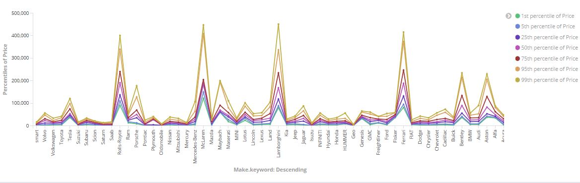
Below is an example of a query which groups similar models and for each of them extracts the average, mininum and maximum price.
Query example
    aggs: {
          Model: {
            aggs: {
              info: {
                stats: {field: "Price"}
              }
            }
            terms: {field: "Model.keyword", size: 10000}
          }
        }
      }
Kibana has been used to create a dashboard in order to visualize the data output of Elasticsearch queries.
Formally, a regression analysis consists of a series of statistical processes aimed at estimating the relationships existing between a set of variables; in particular we try to estimate the relationship between a special variable called dependent (in our case the price) and the remaining independent variables (the other features). This analysis makes it possible to understand how the value of the dependent variable changes as the value of any of the independent variables changes, keeping the others fixed.
To carry out the prediction, various techniques have been studied including linear regression, decision trees and decision tree forests.
Before preprocessing the data we must take a look to how the dataset shows up. In particular we carry out an analysis on the price attribute: describing it allows us to appreciate some informations such as min and max values and standard deviation. We then proceed to compute skewness and kurtosis of the distribution. Next, we observe its relationship with numerical and categorical features by plotting some graphs.
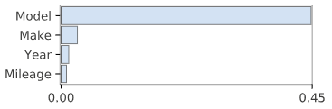
Feature importance computation showed us that Year and Mileage are both important for Price attribute and through correlation matrices we can learn a bit more about that.
The dataset used to carry out the analysis is one of the best available in terms of cleanliness. Despite this, it was necessary to perform preprocessing in order to minimize the probability of incorrect learning by the models.
First it was ascertained that none of the attributes of the dataset presented null values; surprisingly, no feature presented null values, so no action was required to do so. Subsequently, the plausibility of the values for each of the numerical attributes (Price, Imm. Year, Mileage) present in the dataset was verified. We observed some cars with an extremely high mileage and we applied a filter on mileage, taking all cars with a mileage between 5000 and 250000. Moreover, we decided to take only the cars registered between 2008 and 2017 (extremes included) because the majority of the dataset is refers to that particular year range.
Lastly, the distribution of Prices has been normalized by applying a log transformation.
| Price Distribution | Probability Plot |
|---|---|
 |
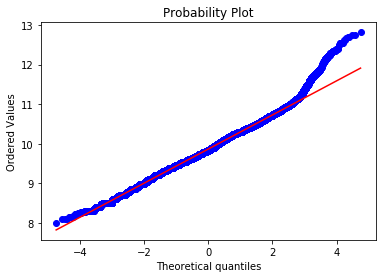 |
As the Car Manufacturer/Price box plot shows, there is a high presence of outliers in the dataset and the only way to tackle this problem is to apply an outliers removal procedure based on the single car model. To do so, we take only the values between the 20th and 80th percentile of the gaussian distribution; this procedure is then applied to each of 3k models.
For managing categorical attributes two different approaches has been taken, depending on the particular regression model.
For linear regression we had to apply a One Hot Encoding(OHE) procedure, through which a noolean attribute is added to the dataset for each unique value of the categorical attributes. Clearly, this procedure must be done with caution because the dimensionality of the set ramps up very quickly.
In our case the only two categorical attributes were Make (car manufacturer) and Model; Model is a categorical variable with more than 3k values and, as mentioned, OHencoding it will generate a dataset with more or less 3000 attributes. That is the technique of choice for linear regressors.
For decision tree and random forests we simply applied a label encoding procedure, through which an increasing number is associated to each value of a categorical attribute. Label Encoding doesn't fit linear regression well because this type of model will try to find a correlation between those values: for example, if Ford is mapped to 501 and BMW is mapped to 650, linear regressors will automatically assume that BMW in a certain way "is better" than Ford.
An advantage of Label Encoding is obviously the fact that the dimensionality remains untouched.
Last but not least, the dataset has been split into training set (66% of total) and hold-out test set (33% of total) for final validation.
In this section we compare the different regression models used in the analysis.
Each of the three prediction models used is characterized by a certain number of parameters (fit_intercept, normalize and copy_X for the linear regressor, max_depth for random forest and decision trees). Based on the value assumed by these parameters, the model may have better / worse performance. The process by which the optimal value is determined for each parameter relative to the training set is called Hyperparameter Tuning.
This is a resource and time-consuming process. The entire project was implemented by exploiting the functionalities offered by the Sci-Kit Learn library (Sklearn) of Python so the parameter tuning process is performed by a function called GridSearchCV: this method performs the fit with every possible combination of parameter values specified in a grid of parameters, executing at the same time the Cross-Validation process that allows to make the most of the available data and reduce the probability of overfitting the model.
To speed up this process, the tuning phase has been carried out exploiting the Spark-Sklearn implementation of GridSearchCV, which uses Apache Spark to parallelize the calculation.
GridSearchCV for Linear Regression applied to the training set outputs these as the best parameters:
LinearRegression(copy_X=True, fit_intercept=False, n_jobs=1, normalize=True)
We then fit a linear regressor with these parameters. In the table below we can observe several information such as scores obtained on training/test sets, Best Score with CV, R2 score and RMSEs.
Using ModelComplexity_DT(X, y) we determine the best value for max_depth parameter. This function fits a Decision Tree Regressor for increasing values of max_depth parameter (values between 10 and 30) and outputs the best value.
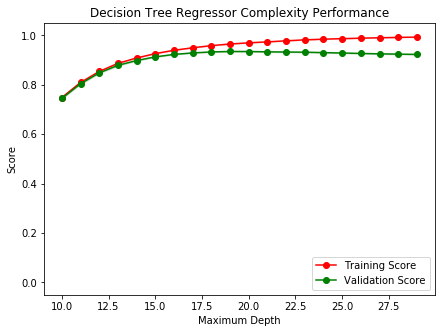
The chart above is called complexity curve and it shows the performance of the model (training and test score) for increasing values of max_depth. The best value is around 17 because the two scores are close; pushing ahead means overfitting the model.
Then, using the method DT_SparkizedGridSearchCV(X, y) we determine precisely which value for max_depth is best.
DecisionTreeRegressor(criterion='mse', max_depth=17, max_features=None,
           max_leaf_nodes=None, min_impurity_decrease=0.0,
           min_impurity_split=None, min_samples_leaf=1,
           min_samples_split=2, min_weight_fraction_leaf=0.0,
           presort=False, random_state=None, splitter='best')
For Random Forest Regressor, ModelComplexity_RF(X, y) plots this complexity curve:
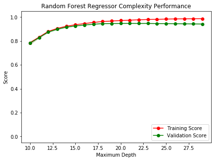
This time we can see that the best value for max_depth is around 18 and to be sure we use RF_SparkizedGridSearchCV(X,y) to determine the best value.
RandomForestRegressor(bootstrap=True, criterion='mse', max_depth=18,
           max_features='auto', max_leaf_nodes=None,
           min_impurity_decrease=0.0, min_impurity_split=None,
           min_samples_leaf=1, min_samples_split=2,
           min_weight_fraction_leaf=0.0, n_estimators=10, n_jobs=1,
           oob_score=False, random_state=None, verbose=0, warm_start=False)
The table below shows experimental results obtained for each model.
| Regression Model | Training Set Score | Test Set Score | Best Score CV=3 | R2 Score | RMSE Training | RMSE Test |
|---|---|---|---|---|---|---|
| Linear | 0.948 | 0.947 | 0.944 | 0.943 | 2361.211 | 2450.764 |
| Decision Tree | 0.949 | 0.930 | 0.931 | 0.911 | 2438.814 | 3080.129 |
| Random Forest | 0.961 | 0.945 | 0.948 | 0.928 | 2204.481 | 2768.085 |
It seems that Linear Regressor achieved the best results since training and test score are very similar to each other and so are RMSEs for training and test. When training's RMSE is much higher than the test one, the model is said to be overfitted. We can see this situation in both decision tree and random forest. Furthermore, linear and random forest regressor's performances are comparable in terms of score, with a small advantage in the best score with CV by Random Forest.
Declaring linear regressor as the winner would be too hasty from us, also because we must not forget that linear regressor in trained with a dataset composed by more or less 3k attributes because of OHE.
Let's observe cross validation results on training set, performed using KFold Cross Validation with K=10.
| Regression Model | S1 | S2 | S3 | S4 | S5 | S6 | S7 | S8 | S9 | S10 | Mean | Std |
|---|---|---|---|---|---|---|---|---|---|---|---|---|
| Linear | 2511.16 | 2507.64 | 2503.01 | 2570.70 | 2837.55 | 2508.55 | 2665.38 | 2564.91 | 2658.98 | 2585.36 | 2591.32 | 100.00 |
| Decision Tree | 2697.16 | 2895.43 | 2876.56 | 3429.01 | 3259.62 | 2809.82 | 3032.75 | 2950.64 | 3517.11 | 2907.55 | 3037.57 | 259.00 |
| Random Forest | 2614.98 | 2581.44 | 2603.29 | 2734.10 | 2908.28 | 2552.35 | 2615.32 | 2829.70 | 2608.75 | 2606.28 | 2665.45 | 112.31 |
Note that these results have been obtained in a certain cross validation session and each of them will produce slightly different results due to the way the dataset is divided in KFold CV method.
As we can see in the cross validation scores table, linear regressor and random forest are the ones that perform better, with a training RMSE of around 2600 and a standard deviation decisively lower than decision tree's one.
Saying that one model is objectively better than another is difficult, especially in this situation where linear regressor is working on a OHencoded dataset and random forest regressor on a label encoded one. Random forests are almost always preferable to linear regressors because they don't need much preprocessing and sometimes they produce good results even in presence of outliers. In our case the differences in performance between linear regressor and random forest are not enough to justify the exaggeratedly high number of attributes introduces by one hot encoding.
Furthermore, random forest regressor fits the data in a fraction of the time required by linear regressor as we can see in the data below:
Linear regressor fit:
CPU times: user 31.7 s, sys: 20.2 s, total: 51.9 s
Wall time: 26.3 s

Random forest regressor fit:
CPU times: user 9.31 s, sys: 9.99 ms, total: 9.32 s
Wall time: 9.33 s
Therefore, Random Forest Regressor has been chosen as the final mode. Following the feature importance computed with K=5 KFold Cross Validaion, scores on the hold-out test set and the final RMSE computed on the entire dataset.
| Regression Model | Test Set Score | R2 Score | RMSE Test |
|---|---|---|---|
| Random Forest | 0.948 | 0.930 | 2747.75 |
| Regression Model | S1 | S2 | S3 | S4 | S5 | S6 | S7 | S8 | S9 | S10 | Mean | Std |
|---|---|---|---|---|---|---|---|---|---|---|---|---|
| Random Forest | 2727.38 | 2520.80 | 2380.93 | 2344.55 | 2417.68 | 2563.77 | 2448.26 | 2609.54 | 2560.65 | 2568.92 | 2514.25 | 110.62 |