scClustMatch

Introduction

Read alignment to a reference genome assembly is an integral component of most single-cell RNA sequencing (scRNAseq) workflows. In an ideal experiment, reads are mapped and aligned to a single "gold standard" reference assembly. Indeed, for well-characterized species with uncontroversial "gold standard" assemblies, such as humans or mice, the use of a single reference remains common practice in single-cell genomics. When a "gold standard" reference for a species is unavailable, however, the researcher is forced to select from an ever-expanding collection of discordant reference assemblies, which vary widely in their completeness and in the quality of their gene annotations. In these cases, reference choice can strongly bias the interpretation of a single-cell dataset, as discordant annotations of cell-type marker genes between variant assemblies can lead to different interpretations of cell-type structure within the same dataset. The result is that clusterings of the same sample may differ sharply depending on which reference assembly is used for read alignment.

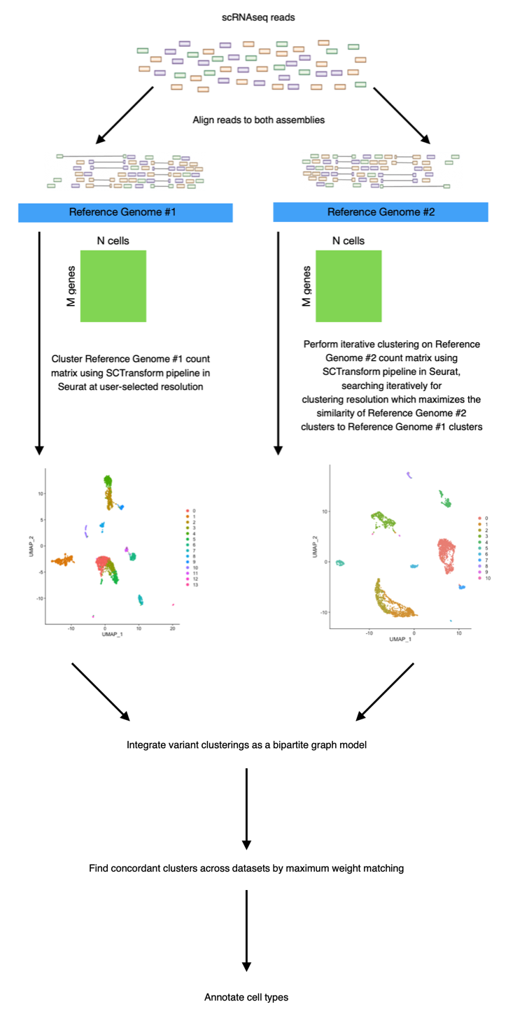
scClustMatch is a data visualization tool for interpreting the effects of reference choice on scRNAseq clustering results. It enables the user to align their reads from a given experiment to multiple candidate reference genomes, and to systematically compare the effects of a particular choice of reference genome on cluster number, size, composition, and coherence. Using a graph-based algorithm (see Appendix), scClustMatch directly compares clusters between variant clusterings, identifying both clusters which are highly conserved (i.e. "matched") regardless of reference choice, and those which can be inferred from one alignment but not the other. In some cases, it may aid the user in identifying distinct cell populations in their data which would not have been detectable using one reference alone. These populations can frequently be identified as cell types whose canonical marker genes are discordantly annotated between variant reference assemblies, or specific to one assembly alone. A typical preparation and workflow for the scClustMatch package is presented as follows:

Installation

scClustMatch can be downloaded from GitHub using the devtools R package:

devtools::install_github("eytan-weinstein/scClustMatch")

Example

In the present example, scClustMatch is used to interpret the effects of reference choice on the clustering of a peripheral blood mononuclear cell (PBMC) single-cell dataset from a healthy woodchuck (Marmota monax). We aligned our dataset to two discordant reference assemblies for the woodchuck: MONAX5 [1] and Woodchuck_1.0 [4], each using the Cell Ranger pipeline from 10x Genomics [6]. The resulting barcodes, features, and count matrix for each alignment were stored in respective directories on a local machine:

MONAX5_directory <- "/Users/eytan/Desktop/Personal/scRNAseq/counts/woodchuck_MONAX5"
list.files(MONAX5_directory)
[1] "barcodes.tsv.gz" "features.tsv.gz" "matrix.mtx.gz" 

Woodchuck_1.0_directory <- "/Users/eytan/Desktop/Personal/scRNAseq/counts/woodchuck_10"
list.files(Woodchuck_1.0_directory)
[1] "barcodes.tsv.gz" "features.tsv.gz" "matrix.mtx.gz"

* For those users wishing to run this example on their own machine, the directories created above are also available for direct download from the cloud via the Dropbox token stored in scClustMatch/inst/testdata/scClustMatch_token.rds. Users can copy the indicated code from scClustMatch/tests/testthat/test-scClustMatch.R in order to import these directories into their own workspace.

In this example, we will consider the MONAX5 assembly to be Reference Genome #1, and the Woodchuck_1.0 assembly to be Reference Genome #2. Our aim will be to investigate how the interpretation of our dataset changes when aligned to Reference Genome #1 vs. Reference Genome #2. The first step in our analysis is to cluster our MONAX5-aligned reads using an appropriate resolution parameter. This resolution parameter is used to select the number of cell-type associated clusters k which we expect to resolve in our Reference Genome #1 clustering. For the sake of simplicity, in this example we will cluster our MONAX5-aligned reads at a relatively coarse resolution of 0.2 (the user may find packages such as Clustree [5] or scClustViz [3] useful for the selection of a suitable resolution parameter in their own analyses). Optionally, we can also specify the PCA dimensions with which to cluster our data (this is set to dims = 30 by default):

MONAX5_clustering <- get_first_clustering(first_directory = MONAX5_directory, reference_resolution = 0.2, dims = 30)

The next step is to cluster our Woodchuck-1.0-aligned reads. Note that we do not select a resolution parameter for our Reference Genome #2 clustering. Instead, scClustMatch will use the resolution parameter from our Reference Genome #1 as a "reference"; clustering the Reference Genome #2 data iteratively in order to select a resolution which maximizes the similarity between the Reference Genome #2 clustering and the Reference Genome #1 clustering generated above:

Woodchuck_1.0_clustering <- get_second_clustering(second_directory = Woodchuck_1.0_directory, first_clustering = MONAX5_clustering)

After both clusterings have been generated, we can see that the clusterings were most similar when resolved at slightly different resolutions:

get_clustering_resolution(MONAX5_clustering)
[1] 0.2

get_clustering_resolution(Woodchuck_1.0_clustering)
[1] 0.27

We can also quantify the maximized similarity between these two clusterings as an adjusted Rand index (ARI) score:

compute_similarity(first_clustering = MONAX5_clustering, second_clustering = Woodchuck_1.0_clustering)
[1] 0.7539969

To compare these clusterings in more detail, we can generate an HTML report to visualize our data in a browser:

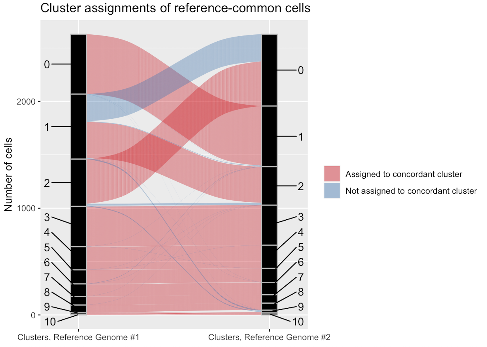
compare_clusterings(first_clustering = MONAX5_clustering, second_clustering = Woodchuck_1.0_clustering)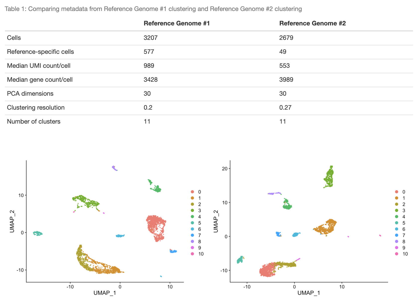

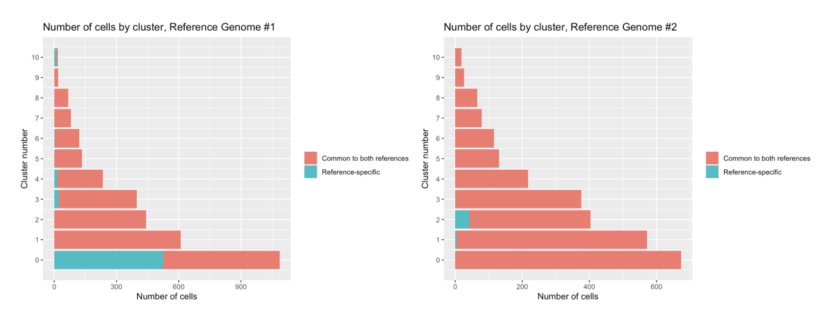
It is clear that in this particular dataset, cell detection is strongly biased by reference choice, as the MONAX5 alignment in particular led to the detection of 577 reference-specific cells. We can also see that these reference-specific cells seem to be disproportionately assigned to Cluster 0 in that alignment.

scClustMatch uses a graph-based algorithm to "match" concordant clusters across both alignments on the basis of pairwise Jaccard similarities between clusters:

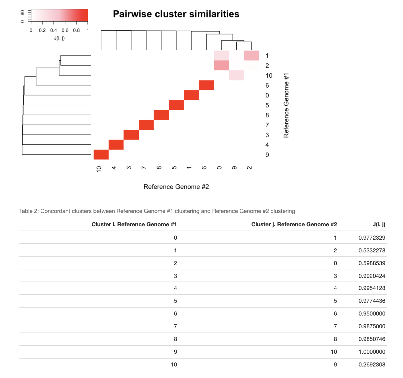
It is important to note that scClustMatch generates the best possible matching. As we can see from the Jaccard similarity scores in Table #2, Cluster 0 in the MONAX5 alignment is highly concordant with its matching Cluster 1 in the Woodchuck_1.0 alignment (when reference-specific cells are discounted), with a Jaccard similarity of 0.9772329. On the other hand, Cluster 10 in the MONAX5 alignment is highly discordant with its best possible match of Cluster 9 in the Woodchuck_1.0 alignment, with a Jaccard similarity of only 0.2692308. In scClustMatch, cluster matchings with low similarity scores usually indicate one of two possible phenomena. First, it is possible that the two clusters, though tentatively matched due to a small degree of overlap, actually correspond to two different cell types. It might just as well be the case, however, that the clusters correspond to the same cell type, but nonetheless include very different populations of cells in the different alignments. The latter phenomenon is common when the marker genes of that conserved cell type are discordantly annotated between variant reference assemblies, leading to false differential expression of those marker genes between the two alignments. To see what is happening in our example, we can extract our data into Seurat [2] in order to perform differential expression testing:

MONAX5_clustering_Seurat <- get_Seurat_object(MONAX5_clustering)
cluster10.markers <- Seurat::FindClusters(MONAX5_clustering_Seurat, ident.1 = 10, logfc.threshold = 0.25, test.use = "roc", only.pos = TRUE)
head(cluster10.markers)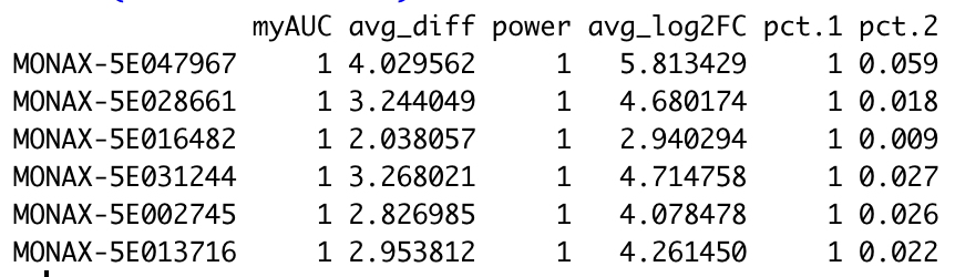

The most significant marker gene of Cluster 10 in the MONAX5 alignment is MONAX-5E047967—the putative woodchuck ortholog of the human platelet factor 4 (PF4). In the Woodchuck_1.0 alignment, the same putative PF4 ortholog is discordantly annotated as GHT09-019442, with a BLAST sequence similarity to MONAX-5E047967 of only 70%. Notably, however, we see that both of these putative PF4 orthologs are significant markers of the matching Clusters 10 and 9 in the MONAX5 and Woodchuck_1.0 alignments, respectively:

Seurat::VlnPlot(MONAX5_clustering_Seurat, features = c("MONAX-5E047967"))
Seurat::VlnPlot(Woodchuck_1.0_clustering_Seurat, features = c("GHT09-019442"))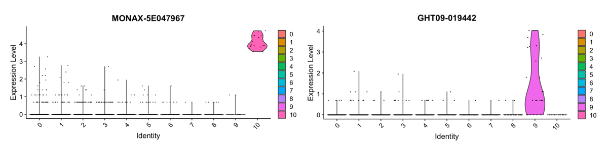

These data suggest that Clusters 10 and 9 were indeed matched correctly by scClustMatch, and likely both correspond to a population of platelets. Nonetheless, false differential expression of the genes MONAX-5E047967 and GHT09-01944 in these two alignments (among other platelet markers) resulted in substantially different groups of cells being assigned to the two respective platelet clusters. As such, the Jaccard similarity between matching Clusters 10 and 9 is quite low (0.2692308) despite their shared identity. A promising integration for this dataset might therefore be the combination of the cells in matching Clusters 10 and 9 into a larger and more accurate platelet cluster, given that reference choice seems to strongly bias the composition of this cluster.

Appendix

A detailed description of the scClustMatch data model and algorithm is presented as follows:

In scClustMatch, maximum weight matching in the bipartite graph G is implemented by the Hungarian algorithm provided with the igraph package.

References

1. Alioto, T.S., Cruz, F., Gómez-Garrido, J. et al. The Genome Sequence of the Eastern Woodchuck (Marmota monax) - A Preclinical Animal Model for Chronic Hepatitis B. G3 9, 12 (2019). https://www.ncbi.nlm.nih.gov/pmc/articles/PMC6893209/
2. Hao, Y., Hao, S., Andersen-Nissen, E. et al. Integrated analysis of multimodal single-cell data. Cell 184, 13 (2021). https://doi.org/10.1101/2020.10.12.335331
3. Innes, B.T., & Bader, G.D. scClustViz - Single-cell RNAseq cluster assessment and visualization. F1000 Research 7, 1522 (2019). https://doi.org/10.12688/f1000research.16198.2
4. Puiu, D., Zimin, A., Shumate, A. et al. The genome of the American groundhog, Marmota monax. F1000 Research 9, 1137 (2020). https://pubmed.ncbi.nlm.nih.gov/33274050/
5. Zappia, L., & Oshlack, A. Clustering trees: a visualization for evaluating clusterings at multiple resolutions. GigaScience 7, 7 (2018). https://academic.oup.com/gigascience/article/7/7/giy083/5052205?login=false
6. Zheng, G., Terry, J., Belgrader, P. et al. Massively parallel digital transcriptional profiling of single cells. Nature Communications 8, 14049 (2017). https://doi.org/10.1038/ncomms14049