dht

Using dht to estimate abundance

Once a detection function has been fitted using the ds function in Distance, one can calculate abundance (and density, though I'll refer only to abundance here for brevity) for some area. Calculating the average probability of detection for each observation, one can use a Horvitz-Thompson estimator to calculate abundance.

Abundance estimates can be calculated either as part of the same call as estimates the detection function (i.e. extra arguments ds) or using the dht function from mrds. Either way one must first create at least two, but maybe three data.frames for region, observation and sample data. We'll begin by talking about these data.frames, before moving on to the two methods for estimating abundace. Finally there is an example of using these approaches.

Note that this page is about the technical details of computing abundance estimates and assumes that the survey has been set up correctly, in particular we are assuming that a (stratified) random sampling design has been used. See Buckland et al (2001) for more information on designing distance sampling surveys.

Setting up data

Two or three additional tables are required to estimate abundance. These define the sample in the context of the wider study area and have a hierarchical relationship.

A note about units: It is important to ensure that all units in this part of the analysis are compatible. If they are not the units of abundance will be incorrect (or at best on a very strange scale). For this reason it is recommended that all units are converted to the metric system before proceeding.

region.table

The region table defines the the overall study region. The data.frame has two columns:

• Region.Label - used to identify the region
• Area - the area of the region

Each row is a strata, if there are no strata then region.table consists of one row: the whole study area.

If lines or points have been replicated, these should be specified in strata (i.e. different Region.Labels).

sample.table

Each row of sample.table specifies a sample -- that is a line or point transect. This data.frame has three columns:

• Region.Label - identifies which region the sample was located in
• Sample.Label - the identifier for this line/point
• Effort - the length of the line/number of times the point was visited

sample.table is linked to the region.table by the Region.Label column.

obs.table

The observation table creates a link between the other two tables and the data used to fit the model (the data.frame used to fit the detection function). If the data used to fit the detection function (the data argument) contains the columns Region.Label and Sample.Label then the obs.table is unnecessary.

If you choose to specify obs.table rather than using data, it must have the following columns:

• object - identifier to a specific observation in data
• Region.Label - identifier for the region
• Sample.Label - identifier for the line or point

The obs.table is linked to the sample.table by the Sample.Label and Region.Label columns.

Using ds to estimate abundance

If you want to estimate abundance in a given area at the same time as fitting the detection function, you can provide region.table and sample.table (and optionally obs.table, as detailed above) to the ds function.

Two additional arguments to ds may also be useful:

• covert.units - gives the conversion factor between the Area, Effort and distance columns. See the "Units" section of the ds manual page for more information.
• dht.group - should estimates of abundance and density set the group size for each observation to be 1 (hence giving the density/abundance of the groups; dht.group=TRUE) or use the observed group size (giving the density/abundance of individuals; dht.group=FALSE).

A simple call to ds may then look like this:

    ds(data, formula=~1, region.table=regions, sample.table=samples)

The disadvantage of this approach is that if one is performing model selection and running several different models (say with different covariates or key functions) each call to ds will take longer as abundance must be calculated each time.

Using dht to estimate abundance

If a detection function has already been fitted, one can call dht separately. As with ds above, the convert.units argument can be used. The equivalent to dht.group above is to supply options=list(group=...), defined as above.

A simple call to dht might look like:

     dht(model$ddf, regions, samples)

where model is a model fitted with ds.

If the detection function was fitted using the ddf function in mrds and was called model then the following is equivalent:

     dht(model, regions, samples)

Example

To show how to take a survey design and put this into the above format, here is a "toy" example. The below image shows a survey area "Region 1" with seven transects (labelled 1-7) and three observations (marked with an "X") on transect 2. (This does not represent a regular distance sampling survey!)

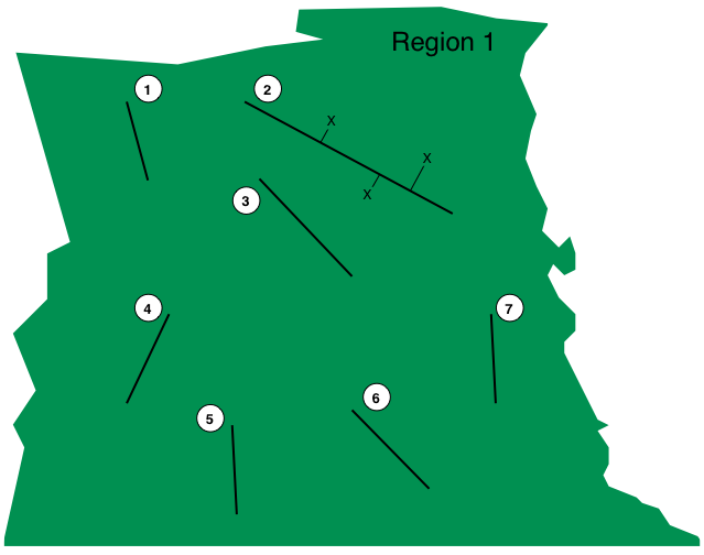
For this survey we would set up the tables as follows:

    regions <- data.frame(Region.Label = 1,
                          Area         = 150)

    samples <- data.frame(Region.Label = rep(1,7),
                          Sample.Label = 1:7,
                          Effort       = c(1,3,1.5,1.2,1,1,0.8))

    data   <- data.frame(distance      = c(0.05,0.1,0.2),
                         object        = 1:3,
                         Region.Label  = rep(1,3),
                         Sample.Label  = rep(2,3))

Assuming that (say) Area is in km^2^ and Effort and distance are in km (distances areas reported here are eyeballed and not the true values!).

References

Buckland, ST, DR anderson, KP Burnham, JL Laake, DL Borchers, and L Thomas. Introduction to Distance Sampling, Oxford University Press, 2001.