Table of contents

• Overview
• CartoDB tutorial
• PostGIS tutorial

Short link to this page

http://bit.ly/car14postgis

Your account

http://LOGIN_NAME.cartodb.com

Overview

This workshop is first and foremost and introduction to PostGIS and the power of geospatial processing with open source tools. To get you there quickly, we are using the CartoDB platform. CartoDB is an open source tool that uses PostGIS to create dynamic interactive maps. CartoDB runs directly in the browser, allowing us to avoid having to install PostGIS during this introduction workshop.

Who

• Andrew Hill, @andrewxhill - Vizzuality
• Michael Keller, @mhkeller - Al Jazeera America, contact info for questions

Bonus

By the end of this workshop you will also have created a map with both Leaflet and Google Maps, you will have created infowindows and legends on an interactive map, and you will have created maps that you can embed and share on your websites or twitter.

Introduction to CartoDB

CartoDB is an open source tool hosted as an online service. Anyone can create a free account and for those more adventurous, the source is available on GitHub.

Tutorials

You can find a long list of tutorials, both written and video, on the CartoDB website

Documentation

As you learn more about CartoDB, start digging into the online documentation

CartoDB allows you to make more than just maps, it can help you build entire geospatial applications. There is an easy to use Javascript library that you can use to integrate maps, geospatial data, and SQL queries into your website.

Support

As you start expirementing more you'll want to know about the GIS StackExchange. If you tag questions with cartodb, postgis or both you will get great help from the community. Just remember to keep question titles short and descriptive. Same goes for the question content, keep it short and to the point. Include links to code (preferably code that wont disappear in the future) or include portions of relevant code for potential helpers to better understand your problem.

Using the dashboard

The CartoDB dashboard is broken down into a few different interfaces.

The table manager

This is the first page you see when you load your account. It is where you will drag new files for upload or create new blank tables. You can see and delete existing datasets here.

The table view

When you load a new dataset or load an old one, you'll be brought to the table view. The table view lets you look at the columns and rows of your data. You can edit individual values. You can change column names and types. You can filter your data and query it using SQL.

Map view

From any table, you can click Map to see the map of the data. As long as your data contained some geospatial information, it should appear on the map. From here, you can style and edit your geospatial data. It is a good place for prototyping published visualizations.

Visualization

Whenever you want to publish a map or combine multiple map layers into a single map to be published, you'll create what is called a Visualization. Visualizations live above maps and tables. They are linked directly to the data in your tables, but you can change the styles and filters of a visualization as much as you like. Visualizations do not take up more space on your account. So from one dataset, you can publish many visualizations.

Visualization manager

Just like your table manager, there is a page for you to see all your visualizations. You can also delete visualizations. Deleting a visualization will not remove the underlying table or map.

Importing data

Importing data into CartoDB is easy! All you need is a file in a supported format (CSV, KML, GeoJSON, and Shapefile are all good ones) either online or on your desktop. You can drag local files right to your browser to import. Remote files you can import by pasting the URL into the import field.

Datasets

File	Dataset name	Geom type
counties_ne.zip	Nebraska Counties	polygons
postoffices_ne.zip	US Post Offices	points

Four ways to get data into CartoDB

1. Drag and drop a file or a ZIP to you dashboard
2. Import from a URL
3. Add new data to a row in your tables or by drawing on the map
4. Use authenticated SQL API calls to write data

First data import

Let's start by importing the dataset of Nebraska Counties.

1. Right click the counties_ne.zip link, copy URL to clipboard
2. Go to your CartoDB dasboard in the table manager
3. Click New table
4. Paste the data URL into the form field
5. Click Create table

Creating maps

Basic map styling

Choropleths, Category maps, Bubble maps

There are many styles possible in CartoDB. The tool includes a simple style wizard for you to apply and customize just some of these. When you grow out of the wizard, you'll want to dig into the CSS editor to really customize your maps.

Infowindows and legends

You can add infowindows and legends to any maps you create. There are some nice simple tools for you to create and customize. As you learn more though, you can also take advantage of full HTML templating to make them look and behave exactly as you want.

Visualizations

Let's start by importing the second dataset of Nebraska Post Offices. Go back to your table manager, then

1. Right click the postoffices_ne.zip link, copy URL to clipboard
2. Go to your CartoDB dasboard in the table manager
3. Click New table
4. Paste the data URL into the form field
5. Click Create table

Now that we have our Post Office dataset, let's create a visualization. You do this by clicking the VISUALIZE button in the upper right. Next, give your visualization a name. This will take you to a new visualization where you can publish you can finalize design, add new layers, or publish your map.

Combine layers

Visualizations allow you to mix multiple datasets into a layered map. You can add a new layer by clicking the plus sign directly above the right-hand menu.

You can reorder the layers on the map by dragging layers up through the stack. Each layer can be styled and edited independantly. You can also add interactivity and legends for the layers.

Publish maps

Right away you can get a public link for your visualization. Where the button VISUALIZE used to be, it should new say PUBLISH. From there you can get the menu for publishing maps.

Links, embeds, CartoDB.js

Publishing maps can be as simple as getting the sharable URL. The interface also gives you an embed option for adding maps to your blog or website. It also has an API option, for using your visualization with our CartoDB.js library. CartoDB.js will allow you to integrate highly customized maps directly into your website. For now, sharable URLs and map embeds should get you pretty far.

PostGIS

PostGIS is an extension for the open-source database PostgreSQL. It's a "spatially-aware" database. For example, let's say you have a spreadsheet with a latitude and a longitude column. To a normal database, those are just numbers. To PostGIS, they are certain places in the world. Knowing that lets you do things like find all points within a certain radius of a given point, or calculate the distance from these points to other things.

Why use PostGIS over ArcMap or QGIS?

• Replicable - you can script your workflow, which is great for leaving a trail of your work.
• It builds on SQL - if you already know SQL, this is an easy way to get into doing GIS analysis.
• You can query data dynamically - if you have a server that can crunch a PostGIS query and return JSON, you can do dynamic spatial queries in your apps. e.g. "Find me all points near me."

Installation

You can install PostGIS locally on your computer by following these guidelines. Since PostGIS is an extension of PostgreSQL, you install PostgreSQL and then activate the PostGIS plugin.

You can also use CartoDB -- like we're doing today -- since CartoDB is in part an interface on top of a PostGIS database. Or you can spin up a PostgreSQL database through Amazon Web Services.

A word of caution: installing PostgreSQL is sometimes no small undertaking and can sometimes be very complicated if the installation doesn't play nicely with your system. Hence, why we're using CartoDB today.

Operators

PostGIS looks a lot like SQL, because it's based on SQL.

• > e.g. SELECT * FROM tbl WHERE year > 1880
• <
• =
• AND
• OR
• IS NULL e.g. SELECT * FROM tbl WHERE year IS NULL
• IS NOT NULL e.g. SELECT * FROM tbl WHERE year IS NOT NULL

Special Operators

Indexed nearest neighbor search. We'll get to this below.

• <->

Filtering, ordering, limiting

Let's start working with historic Post Offices in Nebraska: postoffices_ne.

Click on the SQL tab we can start doing some basic querying.

Filtering: WHERE

SQL can filter using the WHERE command.

SELECT * FROM postoffices_ne WHERE yr_est < 1860

SELECT * FROM postoffices_ne WHERE elev < 400

-- filter by two conditions
SELECT * FROM postoffices_ne WHERE yr_est > 1860 AND yr_est < 1870

-- filter by with an OR
SELECT * FROM postoffices_ne WHERE yr_est > 1890 OR elev < 300

-- More complex OR and AND
SELECT * FROM postoffices_ne WHERE (yr_est > 1870 AND yr_est < 1899) OR elev > 1400

Ordering: ORDER BY

Order by yr_est made

SELECT * FROM postoffices_ne ORDER BY yr_est

SELECT * FROM postoffices_ne ORDER BY yr_est DESC

You can also set ASC for ascending, which is the default.

Limiting: LIMIT

Instead of showing every row, you can limit your query. This can be useful to make your queries faster or decrease the files size of your data export.

Grab the first five

SELECT * FROM postoffices_ne LIMIT 5

This data isn't in any order though, so that query isn't very helpful. This will grab the five oldest.

SELECT * FROM postoffices_ne ORDER BY yr_est LIMIT 5

Or you can grab the five highest

SELECT * FROM postoffices_ne ORDER BY elev DESC LIMIT 5

Selecting, counting

Selecting

We've been doing SELECT statements to create a view on our database. You might have noticed the *, which means "Get all columns". You can also only retrieve specific columns by name.

SELECT county, yr_est, elev FROM postoffices_ne LIMIT 10

Because this is a spatially-aware database, we also have a column that holds our lat/lng. PostGIS usually refers to this column as geom or the_geom in CartoDB.

SELECT county, yr_est, elev, the_geom FROM postoffices_ne LIMIT 10

And we can convert that geometry into different formats

SELECT ST_AsGeoJSon(the_geom), county, yr_est, elev FROM postoffices_ne

BONUS: To make nice column names from aggregate functions, as can alias them with AS.

SELECT ST_AsGeoJSon(the_geom) as geojson, county, yr_est, elev FROM postoffices_ne

Counting

Let's say you want to know some aggregate information, like how many rows you have

SELECT count(*) FROM postoffices_ne

SELECT count(*) FROM postoffices_ne WHERE yr_est > 1880

Spatial joining with ST_Intersects()

Sometimes you join data based on a shared column id. For example, you have a shapefile of police precincts, an Excel file of crime states per precinct and you join them on a shared precinct ID to make a map.

You can do that in CartoDB with the merge tool, but, data doesn't come preaggregated like this. What if you only had the incident data and wanted to make a choropleth showing aggregate counts per polygon?

Let's make a map of Post Office density by county in Nebraska. It might not look that cool, it's probably just a population map, but the concept you can use over and over.

Open up counties_ne and let's add a column, call it, postoffices and set its type to number.

Now, run this query:

UPDATE counties_ne SET postoffices = (
  SELECT count(*) 
  FROM postoffices_ne 
  WHERE 
  ST_Intersects(
    postoffices_ne.the_geom, 
    counties_ne.the_geom 
  )
)

Let's start with the SELECT query first. We're counting the number of Post Offices WHERE the geometries from each table overlap. Put differently, For each county subdivision, count the number of Post Offices that fall within its borders.

Next, add our counties row with that number. That's where the UPDATE query comes in. Usually, it makes most sense to read SQL queries inside out, like math equations.

More generically:

UPDATE name_of_polygon_table SET new_column_name = (
  SELECT count(*) 
  FROM name_of_point_table 
  WHERE 
  ST_Intersects(
    name_of_point_table.the_geom, 
    name_of_polygon_table.the_geom 
  )
)

Note: If you aren't using CartoDB, replace the_geom with geom.

Mapping distance with ST_Distance() and ORDER BY <->

PostGIS is also really powerful for measuring distance, which can be a great story topic. Cezary Podkul did a great story a couple of years ago at Reuters looking at Post Offices that were closing that were also far away from broadband access.

We can do this same calculation right here. We'll measure the distance from each Post Office to the nearest area that has broadband.

Datasets

Import broadband_ne, which shows areas of Nebraska that have broadband access. We're actually going to be doing the measurement in postoffices_ne since that's the data we'll be modifying.

File	Dataset name	Geom type
broadband_ne.zip	Nebraska Broadband areas	polygons

1. Right click the broadband_ne.zip link, copy URL to clipboard
2. Go to your CartoDB dasboard in the table manager
3. Click New table
4. Paste the data URL into the form field
5. Click Create table

Create a new column in postoffices_ne called dist and set its type to number.

UPDATE postoffices_ne SET dist = (
  SELECT ST_Distance(
            postoffices_ne.the_geom::geography, 
            broadband_ne.the_geom::geography
          )
          FROM broadband_ne 
          ORDER BY postoffices_ne.the_geom <-> broadband_ne.the_geom 
          LIMIT 1
)

So, starting from the inside going out, we're ordering our table with this crazy <-> operator, which finds the lat/lng of a Post Office point and sorts the table in ascending order of distance to that point. In other words, take a given post office, and sort the areas in the broadband table in order of increasing distance away from that point -- do that for every post office point.

You can read more about what the <-> does with the indexed-nearest neighbor search.

Now, you can see in the SELECT part, we're then measuring the distance between that Post Office and the areas with broadband. This query would measure the distance from a given post office to every point with broadband but we just want the first one. Because the ORDER BY has already put the closest broadband area first, we just need the measurement to first row, so hence the LIMIT 1.

Now, do the same UPDATE query and add it as our dist column, for every post office.

We're also setting the data type of our geometry column to geography by using ::geography. This ensures that the units of our distance calculation are in meters.

Or more generically:

UPDATE name_of_point_table SET new_column_name = (
  SELECT ST_Distance(
            name_of_point_table.the_geom::geography, 
            name_of_polygon_table.the_geom::geography
          )
          FROM broadband_ne 
          ORDER BY name_of_point_table.the_geom <-> name_of_polygon_table.the_geom 
          LIMIT 1
)

Note: If you aren't using CartoDB, replace the_geom with geom.

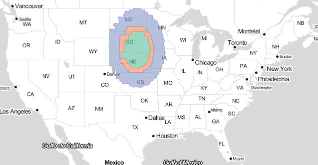
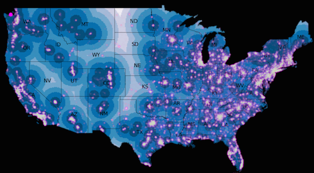
We used this at Al Jazeera America for a story on Syrian refugees showing how much space that many people take up in the US to give context to an international story.

Normalizing counts by area

It can be nice to know how many points fall within a polygon, as we did above in the Spatial Joining section. Sometimes you want to normalize your data to see how your counts compare to something like the population or, in this example, the area of the county subdivision. You can see this is the same as our spatial join query except we're dividing by the value we want to normalize over.

UPDATE counties_ne SET po_density =
      (
        SELECT 
          count(*) 
        FROM 
          postoffices_ne 
        WHERE 
          ST_Intersects(counties_ne.the_geom, the_geom)
      ) / ST_Area(the_geom::geography)

You could also normalize by population

UPDATE counties_ne SET po_density =
      (
        SELECT 
          count(*) 
        FROM 
          postoffices_ne 
        WHERE 
          ST_Intersects(counties_ne.the_geom, the_geom)
      ) / pop_est

More generically:

UPDATE name_of_polygon_data SET new_column_name =
      (
        SELECT 
          count(*) 
        FROM 
          name_of_point_data 
        WHERE 
          ST_Intersects(name_of_polygon_data.the_geom, the_geom)
      ) / name_of_column_to_normalize_over_or_a_postgis_function

Other fun functions

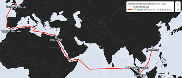
• ST_AsGeoJson() - Convert your geom column to GeoJSON. Useful for exporting your data or returning it to the client web browser to plot using Leaflet.js.
• ST_MakeLine() - Convert points into a line. We used this at Al Jazeera America to scrape a ship's location and then dynamically plot that route.

• ST_Distance() - Measure the distance. We used this at The Daily Beast to create a map of distance away from abortion clinics from every point in the country.

• ST_MakeValid() - If you have errors in your shapefiles, this might fix them.
• ST_DWithin() - Find features that are within a certain specified distance of your feature. E.g. Find all census blocks near a mile of oil wells and add up their populations.
• ST_Buffer() - Draw a circle around a point. Similar but not as powerful as ST_DWithin.
• ST_Intersection() - Similar to Clip in ArcMap: "Returns a geometry that represents the shared portion of geomA and geomB."
• ST_Centroid()) - Get the center point of a polygon. Word of caution: it might not fall within that polygon. For that, try ST_PointOnSurface().

Links, resources

• More about joining data - With spatial joins and normal SQL joins.

• PostGIS Documentation - Read through the functions to see what it's capable of.

• PostGIS Homepage

• PostPostGIS - A Twitter account that discusses geospatial analysis and critical theory.

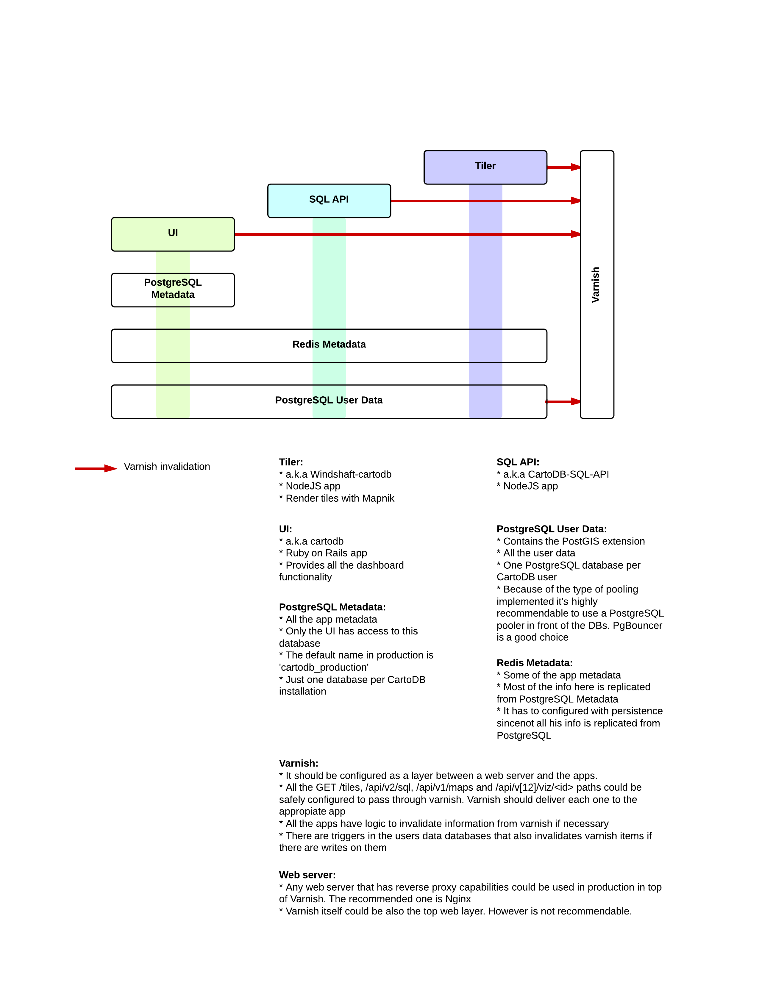
• Luis Bosque at Vizzuality put together this chart showing how the overall CartoDB PostgreSQL/tiler/SQL API/cacheing structure works.