This can construct the tight-binding model and calculate energies in Julia 1.0. This software is released under the MIT License, see LICENSE. We checked that it works in Julia 1.7.
This can
- construct the Hamiltonian as a functional of a momentum k.
- plot the band structure.
- show the crystal structure.
- plot the band structure of the finite-width system with one surface or boundary.
- [09 Feb. 2019] make surface Hamiltonian from the momentum space Hamiltonian.
- [19 Nov. 2019] get DOS data and energy mesh
- [22 Jun. 2020] construct a supercell model
- [EXPERIMENTAL][22 Jun. 2020] write Wannier90 format.
There is the sample jupyter notebook.
Push "]" to enter the package mode.
add TightBinding
Here is a Graphene case
using TightBinding
#Primitive vectors
a1 = [sqrt(3)/2,1/2]
a2= [0,1]
#set lattice
la = set_Lattice(2,[a1,a2])
#add atoms
add_atoms!(la,[1/3,1/3])
add_atoms!(la,[2/3,2/3])
Then we added two atoms (atom 1 and atom 2). We can see the possible hoppings.
show_neighbors(la)Output is
Possible hoppings
(1,1), x:-1//1, y:-1//1
(1,2), x:-2//3, y:-2//3
(2,2), x:-1//1, y:-1//1
(1,1), x:-1//1, y:0//1
(1,2), x:-2//3, y:1//3
(2,2), x:-1//1, y:0//1
(1,1), x:-1//1, y:1//1
(1,2), x:-2//3, y:4//3
(2,2), x:-1//1, y:1//1
(1,1), x:0//1, y:-1//1
(1,2), x:1//3, y:-2//3
(2,2), x:0//1, y:-1//1
(1,1), x:0//1, y:0//1
(1,2), x:1//3, y:1//3
(2,2), x:0//1, y:0//1
(1,1), x:0//1, y:1//1
(1,2), x:1//3, y:4//3
(2,2), x:0//1, y:1//1
(1,1), x:1//1, y:-1//1
(1,2), x:4//3, y:-2//3
(2,2), x:1//1, y:-1//1
(1,1), x:1//1, y:0//1
(1,2), x:4//3, y:1//3
(2,2), x:1//1, y:0//1
(1,1), x:1//1, y:1//1
(2,2), x:1//1, y:1//1
If you want to construct the Graphene, you choose hoppings from atom 1 to atom 2:
#construct hoppings
t = 1.0
add_hoppings!(la,-t,1,2,[1/3,1/3])
add_hoppings!(la,-t,1,2,[-2/3,1/3])
add_hoppings!(la,-t,1,2,[1/3,-2/3])
using Plots
#show the lattice structure
plot_lattice_2d(la)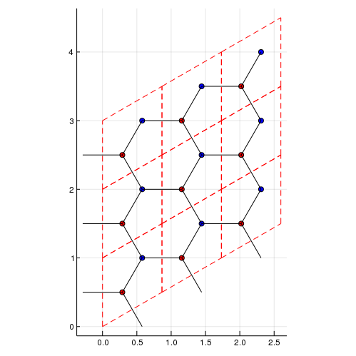
using Plots
# Density of states
nk = 100 #numer ob meshes. nk^d meshes are used. d is a dimension.
plot_DOS(la, nk)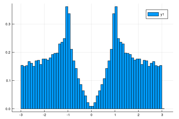
[19 Nov. 2019] We can get DOS data and energy mesh.
nk = 100 #numer ob meshes. nk^d meshes are used. d is a dimension.
hist = get_DOS(la, nk)
println(hist.weights) #DOS data
println(hist.edges[1]) #energy mesh
using Plots
plot(hist.edges[1][2:end] .- hist.edges[1].step.hi/2,hist.weights)#show the band structure
klines = set_Klines()
kmin = [0,0]
kmax = [2π/sqrt(3),0]
add_Kpoints!(klines,kmin,kmax,"G","K")
kmin = [2π/sqrt(3),0]
kmax = [2π/sqrt(3),2π/3]
add_Kpoints!(klines,kmin,kmax,"K","M")
kmin = [2π/sqrt(3),2π/3]
kmax = [0,0]
add_Kpoints!(klines,kmin,kmax,"M","G")
calc_band_plot(klines,la)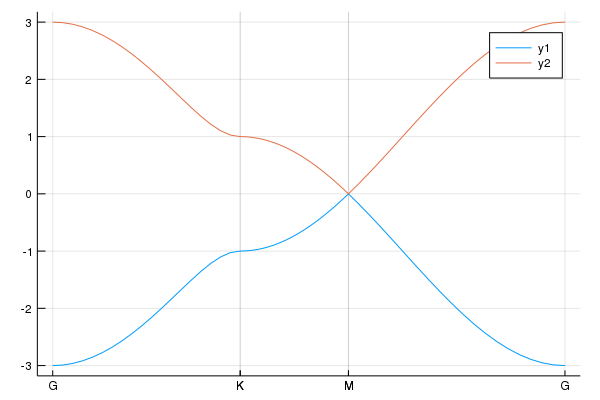
using Plots
#We have already constructed atoms and hoppings.
#We add the line to plot
klines = set_Klines()
kmin = [-π]
kmax = [π]
add_Kpoints!(klines,kmin,kmax,"-pi","pi")#We consider the periodic boundary condition along the primitive vector
direction = 1
#Periodic boundary condition
calc_band_plot_finite(klines,la,direction,periodic=true)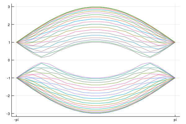
#We introduce the surface perpendicular to the premitive vector
direction = 1
#Open boundary condition
calc_band_plot_finite(klines,la,direction,periodic=false)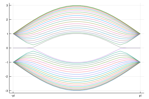
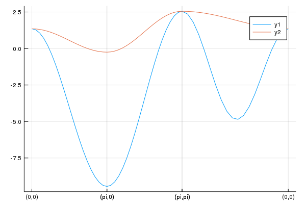
We construct two-band model for Fe-based superconductor [S. Rachu et al. Phys. Rev. B 77, 220503(R) (2008)].
la = set_Lattice(2,[[1,0],[0,1]]) #Square lattice
add_atoms!(la,[0,0]) #dxz orbital
add_atoms!(la,[0,0]) #dyz orbital
#hoppings
t1 = -1.0
t2 = 1.3
t3 = -0.85
t4 = t3
μ = 1.45

#dxz
add_hoppings!(la,-t1,1,1,[1,0])
add_hoppings!(la,-t2,1,1,[0,1])
add_hoppings!(la,-t3,1,1,[1,1])
add_hoppings!(la,-t3,1,1,[1,-1])

#dyz
add_hoppings!(la,-t2,2,2,[1,0])
add_hoppings!(la,-t1,2,2,[0,1])
add_hoppings!(la,-t3,2,2,[1,1])
add_hoppings!(la,-t3,2,2,[1,-1])

#between dxz and dyz
add_hoppings!(la,-t4,1,2,[1,1])
add_hoppings!(la,-t4,1,2,[-1,-1])
add_hoppings!(la,t4,1,2,[1,-1])
add_hoppings!(la,t4,1,2,[-1,1])

#Chemical potentials
set_μ!(la,μ) #set the chemical potential
To see the band structure, we use
klines = set_Klines()
kmin = [0,0]
kmax = [π,0]
add_Kpoints!(klines,kmin,kmax,"(0,0)","(pi,0)")

kmin = [π,0]
kmax = [π,π]
add_Kpoints!(klines,kmin,kmax,"(pi,0)","(pi,pi)")

kmin = [π,π]
kmax = [0,0]
add_Kpoints!(klines,kmin,kmax,"(pi,pi)","(0,0)")

using Plots
pls = calc_band_plot(klines,la)
Then, we have the band structure:
We can obtain the Hamiltonian:
ham = hamiltonian_k(la) #we can obtain the function "ham([kx,ky])".
kx = 0.1
ky = 0.2
hamk = ham([kx,ky]) #ham is a functional of k=[kx,ky].
println(hamk)Finally, we show the 5-orbital model proposed by K. Kuroki et al.[K. Kuroki et al., Phys. Rev. Lett. 101, 087004 (2008)]. The sample code is
la = set_Lattice(2,[[1,0],[0,1]])
add_atoms!(la,[0,0])
add_atoms!(la,[0,0])
add_atoms!(la,[0,0])
add_atoms!(la,[0,0])
add_atoms!(la,[0,0])

tmat = [
-0.7    0 -0.4  0.2 -0.1
-0.8    0    0    0    0
 0.8 -1.5    0    0 -0.3
   0  1.7    0    0 -0.1
-3.0    0    0 -0.2    0
-2.1  1.5    0    0    0
 1.3    0  0.2 -0.2    0
 1.7    0    0  0.2    0
-2.5  1.4    0    0    0
-2.1  3.3    0 -0.3  0.7
 1.7  0.2    0  0.2    0
 2.5    0    0  0.3    0
 1.6  1.2 -0.3 -0.3 -0.3
   0    0    0 -0.1    0
 3.1 -0.7 -0.2    0    0
]
tmat = 0.1.*tmat
imap = zeros(Int64,5,5)
count = 0
for μ=1:5
    for ν=μ:5
        count += 1
        imap[μ,ν] = count
    end
end
Is = [1,-1,-1,1,1,1,1,-1,-1,1,-1,-1,1,1,1]
σds = [1,-1,1,1,-1,1,-1,-1,1,1,1,-1,1,-1,1]
tmat_σy = tmat[:,:]
tmat_σy[imap[1,2],:] = -tmat[imap[1,3],:]
tmat_σy[imap[1,3],:] = -tmat[imap[1,2],:]
tmat_σy[imap[1,4],:] = -tmat[imap[1,4],:]
tmat_σy[imap[2,2],:] = tmat[imap[3,3],:]
tmat_σy[imap[2,4],:] = tmat[imap[3,4],:]
tmat_σy[imap[2,5],:] = -tmat[imap[3,5],:]
tmat_σy[imap[3,3],:] = tmat[imap[2,2],:]
tmat_σy[imap[3,4],:] = tmat[imap[2,4],:]
tmat_σy[imap[3,5],:] = -tmat[imap[2,5],:]
tmat_σy[imap[4,5],:] = -tmat[imap[4,5],:]

hoppingmatrix = zeros(Float64,5,5,5,5)
hops = [-2,-1,0,1,2]
hopelements = [[1,0],[1,1],[2,0],[2,1],[2,2]]

for μ = 1:5
    for ν=μ:5
        for ii=1:5
            ihop = hopelements[ii][1]
            jhop = hopelements[ii][2]
            #[a,b],[a,-b],[-a,-b],[-a,b],[b,a],[b,-a],[-b,a],[-b,-a]

            #[a,b]
            i = ihop +3
            j = jhop +3
            hoppingmatrix[μ,ν,i,j]=tmat[imap[μ,ν],ii]
            #[a,-b] = σy*[a,b] [1,1] -> [1,-1]
            if jhop != 0
                i = ihop +3
                j = -jhop +3
                hoppingmatrix[μ,ν,i,j]=tmat_σy[imap[μ,ν],ii]
            end

            if μ != ν
                #[-a,-b] = I*[a,b] [1,1] -> [-1,-1],[1,0]->[-1,0]
                i = -ihop +3
                j = -jhop +3
                hoppingmatrix[μ,ν,i,j]=Is[imap[μ,ν]]*tmat[imap[μ,ν],ii]
                #[-a,b] = I*[a,-b] = I*σy*[a,b]  #[2,0]->[-2,0]
                if jhop != 0
                    i = -ihop +3
                    j = jhop +3
                    hoppingmatrix[μ,ν,i,j]=Is[imap[μ,ν]]*tmat_σy[imap[μ,ν],ii]
                end
            end
            #[b,a],[b,-a],[-b,a],[-b,-a]
            if jhop != ihop
                #[b,a] = σd*[a,b]
                i = jhop +3
                j = ihop +3
                hoppingmatrix[μ,ν,i,j]=σds[imap[μ,ν]]*tmat[imap[μ,ν],ii]
                #[-b,a] = σd*σy*[a,b]
                if jhop != 0
                    i = -jhop +3
                    j = ihop +3
                    hoppingmatrix[μ,ν,i,j]=σds[imap[μ,ν]]*tmat_σy[imap[μ,ν],ii]
                end

                if μ != ν
                    #[-b,-a] = σd*[-a,-b] = σd*I*[a,b]
                    i = -jhop +3
                    j = -ihop +3
                    hoppingmatrix[μ,ν,i,j]=σds[imap[μ,ν]]*Is[imap[μ,ν]]*tmat[imap[μ,ν],ii]
                    #[b,-a] = σd*[-a,b] = σd*I*[a,-b] = σd*I*σy*[a,b]  #[2,0]->[-2,0]
                    if jhop != 0
                        i = jhop +3
                        j = -ihop +3
                        hoppingmatrix[μ,ν,i,j]=σds[imap[μ,ν]]*Is[imap[μ,ν]]*tmat_σy[imap[μ,ν],ii]
                    end
                end
            end
        end


    end
end

for μ=1:5
    for ν=μ:5
        for i = 1:5
            ih = hops[i]
            for j = 1:5
                jh = hops[j]
                if hoppingmatrix[μ,ν,i,j] != 0.0
                    add_hoppings!(la,hoppingmatrix[μ,ν,i,j],μ,ν,[ih,jh])
                end
            end
        end
    end
end

onsite = [10.75,10.96,10.96,11.12,10.62]
set_onsite!(la,onsite)

set_μ!(la,10.96) #set the chemical potential
Then, we plot the band structure
nk = 100
klines = set_Klines()
kmin = [0,0]
kmax = [π,0]
add_Kpoints!(klines,kmin,kmax,"(0,0)","(pi,0)",nk=nk)

kmin = [π,0]
kmax = [π,π]
add_Kpoints!(klines,kmin,kmax,"(pi,0)","(pi,pi)",nk=nk)

kmin = [π,π]
kmax = [0,0]
add_Kpoints!(klines,kmin,kmax,"(pi,pi)","(0,0)",nk=nk)

using Plots
pls = calc_band_plot(klines,la)
savefig("Fe5band.png")
We have the band structure:
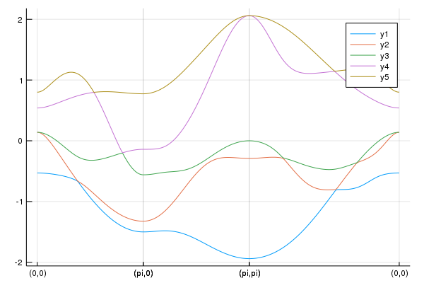
This figure is consistent with Fig.2 in the paper where the hopping table is used [T. Nomura, J. Phys. Soc. Jpn. 78, 034716 (2009)].
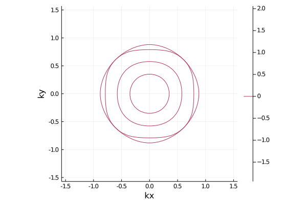
The Fermi surface is given by
pls = plot_fermisurface_2D(la)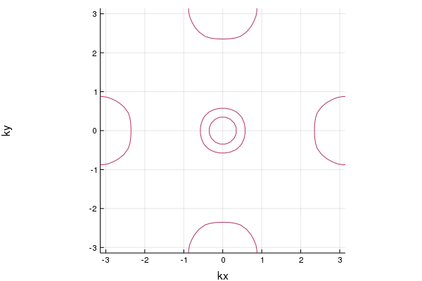
If we have the Hamiltonian defined in momentum space, we can construct the surface Hamiltonian. For example, we consider a model of 2D topological insulator:
using TightBinding
Ax = 1
Ay = 1
m2x = 1
m2y = m2x
m0 = -2*m2x
m(k) = m0 + 2m2x*(1-cos(k[1]))+2m2y*(1-cos(k[2]))
Hk(k) = Ax*sin(k[1]).*σx +  Ay*sin(k[2]).*σy + m(k).*σz
norb = 2 #The size of the matrix
Now, when you use TightBinding.jl, the Pauli matrices σx,σy,σz,σ0 are defined. Then,
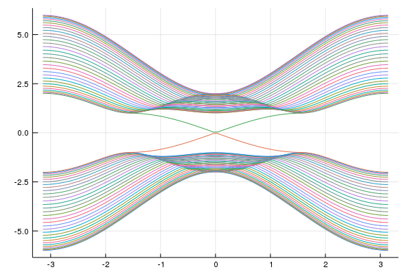
hamiltonian = surfaceHamiltonian(Hk,norb,numhop=3,L=32,kpara="kx",BC="OBC")makes the function hamiltonian(k). We can choose open boundary condition OBC or periodic boundary condition PBC. numhop determines the number of the maximum hoppings. numhop-th nearest neighbor hopping can be included. L detemines the size of the real space lattice.
using Plots
using LinearAlgebra
nkx = 100
kxs = range(-π,stop=π ,length=nkx)
mat_e = zeros(Float64,nkx,32*2)
for i=1:nkx
    kx = kxs[i]
    mat_h = hamiltonian(kx)
    #println(mat_h)

    e,v = eigen(Matrix(mat_h))
    #println(e)
    mat_e[i,:] = real.(e[:])
end
plot(kxs,mat_e,labels="")
savefig("tes1.png")
You can see the surface state.
We can construct supercell model.
We make the graphene:
using TightBinding
#Primitive vectors
a1 = [sqrt(3)/2,1/2]
a2= [0,1]
#set lattice
la = set_Lattice(2,[a1,a2])
#add atoms
add_atoms!(la,[1/3,1/3])
add_atoms!(la,[2/3,2/3])

#construct hoppings
t = 1.0
add_hoppings!(la,-t,1,2,[1/3,1/3])
add_hoppings!(la,-t,1,2,[-2/3,1/3])
add_hoppings!(la,-t,1,2,[1/3,-2/3])
Then, use make_supercell command:
la_2x2 = make_supercell(la,[2,2])Then, you can have the supercell model:
using Plots
#show the lattice structure
plot_lattice_2d(la_2x2)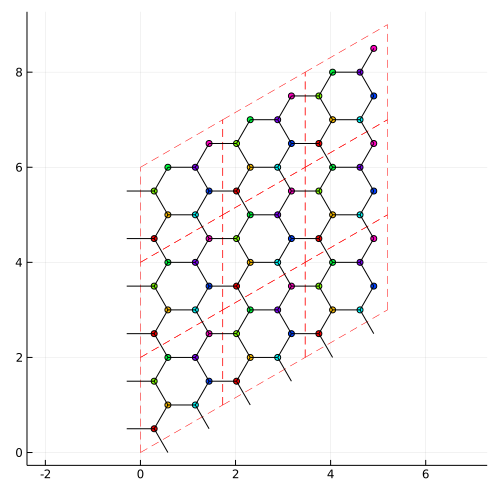
The density of states is same:
# Density of states
nk = 100 #numer ob meshes. nk^d meshes are used. d is a dimension.
plot_DOS(la_2x2, nk)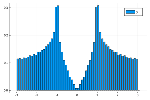
You can write the wannier90 file format. Wannier90 is in here It might be useful to have the wannier90_hr format.
    la2 = set_Lattice(2,[[1,0],[0,1]])
    add_atoms!(la2,[0,0])

    show_neighbors(la2)

    t = 1.0
    add_hoppings!(la2,-t,1,1,[1,0])
    add_hoppings!(la2,-t,1,1,[0,1])
    ham2 = hamiltonian_k(la2)

    kmin = [-π,-π]
    kmax = [0.0,0.0]
    nk = 20
    vec_k,energies = calc_band(kmin,kmax,nk,la2,ham2)
    println("Energies on the line from (-π,π) to (0,0)")
    println(energies)

    las = make_supercell(la2,[2,2])
    ham2s = hamiltonian_k(las)

    vec_ks,energiess = calc_band(kmin,kmax,nk,las,ham2s)
    println("Energies on the line from (-π,π) to (0,0)")
    println(energiess)

    write_hr(la2,filename="2dsample_hr.dat")
    write_hr(las,filename="2dsample_sp_hr.dat")
write_hr function writes a Lattice type struct as wannier90_hr.dat format
You can read the wannier90_hr format. For example, we write the wannier90 format for 5-band Fe-based superconductor as shown above. Then, we have la as Lattice type. We build a supercell for example.
las = make_supercell(la,[2,2])Then, write las as the wannier90_hr format.
write_hr(las,filename="pnictide_5band_2x2_hr.dat")In the wannier90 format, there is no information about lattice vectors and positions of atoms. We have to define these before reading the file. So we make new Lattice type. In our example, the lattice vectors are [2,0] and [0,2]. So, we add
la_new = set_Lattice(2,[[2,0],[0,2]])and there 20 atoms whose positions are
println(las.positions)[[0.0, 0.0], [0.0, 0.0], [0.0, 0.0], [0.0, 0.0], [0.0, 0.0], [0.5, 0.0], [0.5, 0.0], [0.5, 0.0], [0.5, 0.0], [0.5, 0.0], [0.0, 0.5], [0.0, 0.5], [0.0, 0.5], [0.0, 0.5], [0.0, 0.5], [0.5, 0.5], [0.5, 0.5], [0.5, 0.5], [0.5, 0.5], [0.5, 0.5]]
We add these information to la_new.
atoms = [[0.0, 0.0], [0.0, 0.0], [0.0, 0.0], [0.0, 0.0], [0.0, 0.0], [0.5, 0.0], [0.5, 0.0], [0.5, 0.0], [0.5, 0.0], [0.5, 0.0], [0.0, 0.5], [0.0, 0.5], [0.0, 0.5], [0.0, 0.5], [0.0, 0.5], [0.5, 0.5], [0.5, 0.5], [0.5, 0.5], [0.5, 0.5], [0.5, 0.5]]
for i=1:20
    add_atoms!(la_new,atoms[i])
end
And set the chemical potential
set_μ!(la_new,10.96)If you do not set the chemical potential, the chemical potential is zero.
Then, we read the wannir90 format file.
la_new = read_wannier(la_new,"pnictide_5band_2x2_hr.dat")After reading it, you can plot Fermi surface etc.
plot_fermisurface_2D(la_new)