


Check out the paper!
You can explore the BIONIC integrated yeast features at https://bionicviz.com/.
See here for the implementation of the co-annotation prediction, module detection, and gene function prediction evaluations.
See here for the implementation of the analyses used to generate the manuscript figures.
BIONIC (Biological Network Integration using Convolutions) is a deep-learning based biological network integration algorithm that incorporates graph convolutional networks (GCNs) to learn integrated features for genes or proteins across input networks. BIONIC produces high-quality gene features and is scalable both in the number of networks and network size.
An overview of BIONIC can be seen below.
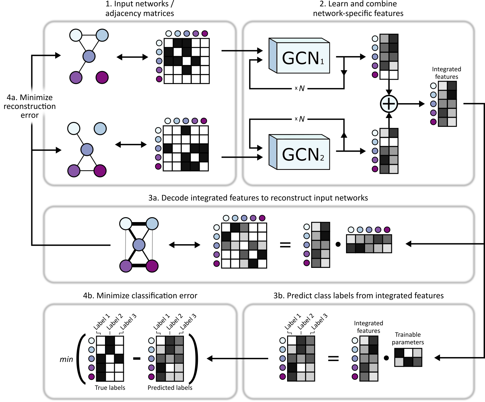
- Multiple networks are input into BIONIC
- Each network is passed through its own graph convolutional encoder where network-specific gene (node) features are learned based the network topologies. These features can be passed through the encoder multiple times to produce gene features which incorporate higher-order neighborhoods. These features are summed to produce integrated gene features which capture topological information across input networks. The integrated features can then be used for downstream tasks, such as gene co-annotation prediction, module detection (via clustering) and gene function prediction (via classification).
- In order to train and optimize the integrated gene features, BIONIC first decodes the integrated features into a reconstruction of the input networks (a) and, if labelled data is available for some of the genes (such as protein complex membership, Gene Ontology annotations, etc.), BIONIC can also attempt to predict these functional labels (b). Note that any amount of labelled data can be used, from none (fully unsupervised), to labels for every gene, and everything in between.
- BIONIC then minimizes the difference between the network reconstruction and the input networks (i.e. reconstruction error) by updating its weights to learn gene features that capture relevant topological information (a) and, if labelled data is provided, BIONIC updates its weights to minimizes the difference between the label predictions and true labels (b).
-
BIONIC is implemented in Python 3.8 and uses PyTorch and PyTorch Geometric.
-
BIONIC can run on the CPU or GPU. The CPU distribution will get you up and running quickly, but the GPU distributions are significantly faster for large models (when run on a GPU), and are recommended.
We provide wheels for the different versions of BIONIC, CUDA, and operating systems as follows:
BIONIC 0.2.0+ (Latest is
cpu |
cu92 |
cu101 |
cu102 |
cu111 |
|
|---|---|---|---|---|---|
| Linux | ✔️ | ✔️ | ✔️ | ||
| Windows | ✔️ | ✔️ | ✔️ |
BIONIC 0.1.0
cpu |
cu92 |
cu101 |
cu102 |
cu111 |
|
|---|---|---|---|---|---|
| Linux | ✔️ | ✔️ | ✔️ | ✔️ | |
| Windows | ✔️ | ✔️ | ✔️ |
NOTE: If you run into any problems with installation, please don't hesitate to open an issue.
If you are installing a CUDA capable BIONIC wheel (i.e. not CPU), first ensure you have a CUDA capable GPU and the drivers for your GPU are up to date. Then, if you don't have CUDA installed and configured on your system already, download, install and configure a BIONIC compatible CUDA version. Nvidia provides detailed instructions on how to do this for both Linux and Windows.
-
Before installing BIONIC, it is recommended you create a virutal Python 3.8 environment using tools like the built in
venvcommand, or Anaconda. -
Make sure your virtual environment is active, then install BIONIC by running
$ pip install https://github.com/bowang-lab/BIONIC/releases/download/v${VERSION}/bionic_model-${VERSION}+${CUDA}-cp38-cp38-${OS}.whlwhere
${VERSION},${CUDA}and${OS}correspond to the BIONIC version, valid CUDA version (as specified above), and operating system, respectively.${OS}takes a value oflinux_x86_64for Linux, andwin_amd64for Windows.For example, if we wanted to install the latest version of BIONIC to run on the CPU on a Linux system, we would run
$ pip install https://github.com/bowang-lab/BIONIC/releases/download/v0.2.6/bionic_model-0.2.6+cpu-cp38-cp38-linux_x86_64.whlNOTE: There is a known bug in certain versions of
pipwhich may result in aNo matching distributionerror. If this occurs, installpip==19.3.1and try again. -
Test BIONIC is installed properly by running
$ bionic --helpYou should see a help message.
-
If you don't already have it, install Poetry.
-
Create a virtual Python 3.8 environment using tools like the built in
venvcommand, or Anaconda. Make sure your virutal environment is active for the following steps. -
Install PyTorch 1.9.0 for your desired CUDA version as follows:
$ pip install torch==1.9.0+${CUDA} -f https://download.pytorch.org/whl/torch_stable.htmlwhere
${CUDA}is the one of the options listed in the table above. -
Install PyTorch 1.9.0 compatible PyTorch Geometric dependencies for your desired CUDA version as follows:
$ pip install torch-scatter==2.0.8 torch-sparse==0.6.11 torch-cluster==1.5.9 -f https://pytorch-geometric.com/whl/torch-1.9.0+${CUDA}.html
$ pip install torch-geometric==1.7.2
where
${CUDA}is the one of the options listed in the table above. -
Clone this repository by running
$ git clone https://github.com/bowang-lab/BIONIC.git -
Make sure you are in the root directory (same as
pyproject.toml) and run$ poetry install -
Test BIONIC is installed properly by running
$ bionic --helpYou should see a help message.
BIONIC runs by passing in a configuration file: a JSON file containing all the relevant model file paths and hyperparameters. You can have a uniquely named config file for each integration experiment you want to run. An example config file can be found here.
The configuration keys are as follows:
| Argument | Default | Description |
|---|---|---|
net_names |
null |
List of filepaths of input networks. If a string is used instead with a "*" after the path, BIONIC will integrate all networks in the corresponding directory. |
label_names |
null |
Filepaths of node label JSON files. An example node label file can be found here. |
out_name |
config file path | Path to prepend to all output files. If not specified it will be the path of the config file. out_name takes the format path/to/output where output is an extensionless output file name. |
delimiter |
" " |
Delimiter for input network files. |
epochs |
3000 |
Number of training steps to run BIONIC for (see usage tips). |
batch_size |
2048 |
Number of genes in each mini-batch. Higher numbers result in faster training but also higher memory usage. |
sample_size |
0 |
Number of networks to batch over (0 indicates all networks will be in each mini-batch). Higher numbers (or 0) result in faster training but higher memory usage. |
learning_rate |
0.0005 |
Learning rate of BIONIC. Higher learning rates result in faster convergence but run the risk of unstable training (see usage tips). |
embedding_size |
512 |
Dimensionality of the learned integrated gene features (see usage tips). |
shared_encoder |
false |
Whether to use the same graph attention layer (GAT) encoder for all the input networks. This may lead to better performance in certain circumstances. |
initialization |
"kaiming" |
Weight initialization scheme. Valid options are "xavier" or "kaiming". |
lambda |
null |
Relative weighting between reconstruction and classification loss: final_loss = lambda * rec_loss + (1 - lambda) * cls_loss. Only relevant if label_names is specified. If lambda is not provided but label_names is, lambda will default to 0.95. |
neighbor_sample_size |
2 |
Size of neighborhoods to sample around each node for progressive GAT passes per training step (see usage tips). |
gat_shapes.dimension |
64 |
Dimensionality of each individual GAT head (see usage tips). |
gat_shapes.n_heads |
10 |
Number of attention heads for each network-specific GAT. |
gat_shapes.n_layers |
2 |
Number of times each network is passed through its corresponding GAT. This number corresponds to the effective neighbourhood size of the convolution. |
model_parallel |
false |
Whether to distribute the model over multiple GPUs (i.e. model parallelism, not data parallelism). This is useful if you have many large networks and a highly parameterized model that will not fit on a single GPU. |
save_network_scales |
false |
Whether to save the internal learned network features scaling coefficients. |
save_label_predictions |
false |
Whether to save the predicted node labels (if applicable). |
save_model |
true |
Whether to save the trained model parameters and state. |
pretrained_model_path |
null |
Path to a pretrained model (.pt file) to load parameters from. |
tensorboard.training |
false |
Whether to output training progress to TensorBoard. |
tensorboard.embedding |
false |
Whether to embed learned feature with TensorBoard projector. |
tensorboard.log_dir |
null |
Output directory of TensorBoard logging files. Default is "runs". See here for more information. |
tensorboard.comment |
"" |
Comment to add to TensorBoard output file name. See here for more information. |
plot_loss |
true |
Whether to plot the model loss curves after training. |
save_loss_data |
false |
Whether to save the training loss data in a .tsv file. |
The . notation indicates a nested field, so gat_shapes.dimension (for example) becomes
gat_shapes: {
    dimension: ${DIM_VALUE}
}
in the config file. By default, only the net_names key is required, though it is recommended you experiment with different hyperparameters to suit your needs.
Input networks are text files in edgelist format, where each line consists of two gene identifiers and (optionally) the weight of the edge between them, for example:
geneA geneB 0.8
geneA geneC 0.75
geneB geneD 1.0
If the edge weight column is omitted, the network is considered binary (i.e. all edges will be given a weight of 1). The gene identifiers and edge weights are delimited with spaces by default. If you have network files that use different delimiters, this can be specified in the config file by setting the delimiter key.
BIONIC assumes all networks are undirected and enforces this in its preprocessing step.
To run BIONIC, do
$ bionic path/to/your_config_file.json
Results will be saved in the out_name directory as specified in the config file.
By default, BIONIC will output loss curves at the end of training if plot_loss is set to true in the config. TensorBoard provides additional functionality over static loss plots (such as organizing different model runs, real-time training metrics, and interactive loss plots) and also allows for visualization of the learned features using TensorFlow Projector.
To use TensorBoard with BIONIC, specify tensorboard.training and/or tensorboard.embedding to be true in the config. You can view the training results by running
$ tensorboard --logdir=path/to/log_files
and navigating to http://localhost:6006/ in your browser. More information on running TensorBoard can be found here.
The configuration parameters table provides usage tips for many parameters. Additional suggestions are listed below. If you have any questions at all, please open an issue.
learning_rateandepochshave the largest effect on training time and performance.learning_rateshould generally be reduced as you integrate more networks. If the model loss suddenly increases by an order of magnitude or more at any point during training, this is a signlearning_rateneeds to be lowered.epochsshould be increased as you integrate more networks. 10000-15000 epochs is not unreasonable for 50+ networks.embedding_sizedirectly affects the quality of learned features. We found the default512works for most networks, though it's worth experimenting with different sizes for your application. In general, higherembedding_sizewill encode more information present in the input networks but at the risk of also encoding noise.gat_shapes.dimensionshould be increased for networks with many nodes. We found128-256is a good size for human networks, for example.- Small values for
neighbor_sample_sizetend to work better than large values.
- BIONIC runs faster and performs better with sparser networks - as a general rule, try to keep the average node degree below 50 for each network.