In this sample project, we look for church buildings in the center of Rome and try to connect them to our bibliographic and photographic holdings - using the common GND entitiy.
The starting point are the churches themselves. Since we don't have direct access to the municipal cataster (which BTW is not as updated as one would like) we use the OpenStreetMap data. That way, we have vector data we can freely use (and abuse) and publish!
If anyone is still unsure about OpenStreetMap: it's the global mapping initiative started in 2004 with now over 10 Million contributors, and updates every minute. Everything is covered by the Open Database license, similar to the Creative Commons SA-BY.
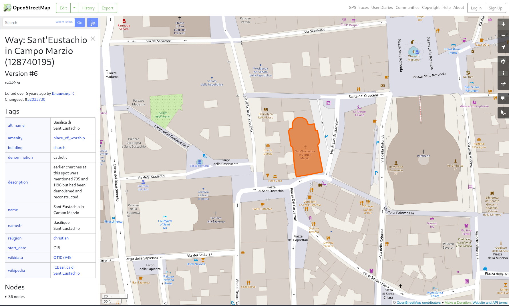
The Openstreetmap way of mapping is by way of Nodes, Ways and Relations: points, polyons and multipolygons in technical speak.
Let's have a look at for example the church of Sant’Eustachio in Campo Marzio:
https://www.openstreetmap.org/way/128740195#map=19/41.89865/12.47573
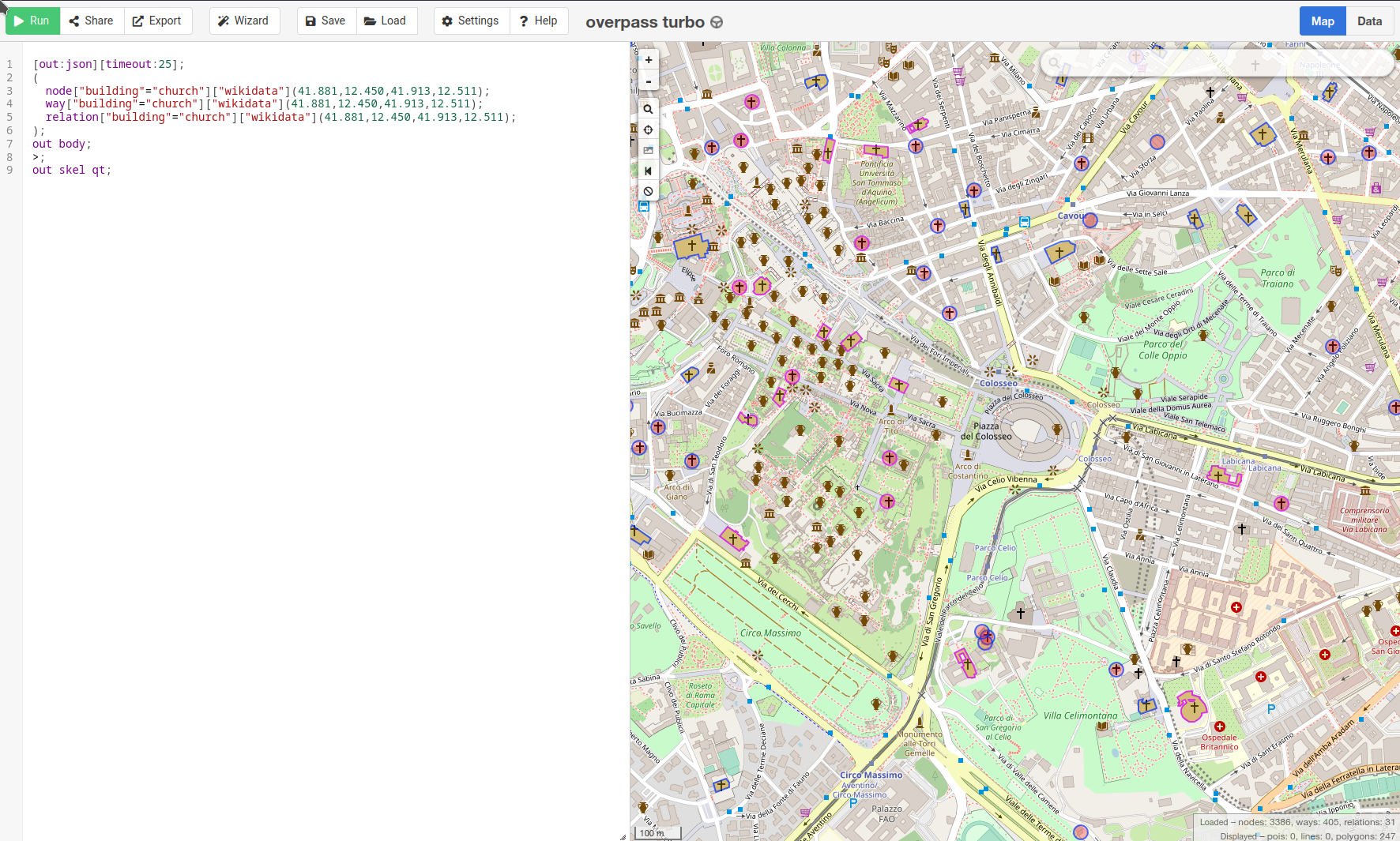
Since OpenStreetMap is at the heart a giant database in PostGreSQL we can easily make a query and get the relative polygons. We use the Overpass editor: https://overpass-turbo.eu/
In the Overpass query we use 3 filters:
-
a bounding box of South 41.881, West 12.450, North 41.913, East 12.511
-
the parameter
buildings=churchin order to filter out the crap like kiosks, bars, restaurants -
the parameter
wikidatain order to ignore all churches without wikidata ID - because we wouldn't be able to connect these to Wikidata anyway.
[out:json][timeout:25];
(
  node["building"="church"]["wikidata"](41.881,12.450,41.913,12.511);
  way["building"="church"]["wikidata"](41.881,12.450,41.913,12.511);
  relation["building"="church"]["wikidata"](41.881,12.450,41.913,12.511);
);
out body;
>;
out skel qt;
We get about 270 records as output in geoJSON.
Save the file (menu: Export / Data / GeoJSON / Download) as export.geojson.
As you see, most of them (about 250) have a wikidata ID:
{
  "type": "FeatureCollection",
  "generator": "overpass-ide",
  "timestamp": "2023-02-22T14:03:38Z",
  "features": [
    {
      "type": "Feature",
      "properties": {
        "@id": "relation/326080",
        "addr:city": "Roma",
        "addr:street": "Via Labicana",
        "amenity": "place_of_worship",
        "building": "church",
        "denomination": "catholic",
        "historic": "church",
        "name:cs": "Bazilika svatého Klimenta v Lateráně",
        "name:en": "Basilica of St.Clement",
        "religion": "christian",
        "type": "multipolygon",
        "wikidata": "Q385910",
        "wikipedia": "it:Basilica di San Clemente al Laterano"
      },
      "geometry": {
        "type": "Polygon",
        "coordinates": [
          [
            [
              12.4980001,
              41.8893645
            ],
            [
              12.4979808,
              41.8893013
            ],
            [
              12.4979449,
              41.8891838
            ],
            [ ... ]
          ]
        ]
      }
   ]
}
They don‹t have a GND ID … that would be too much to ask for … but we get this vital ID in the second step from Wikidata!
In order to get the GND ID - which we need to connect the vectors form Openstreetmap with our institutional databases - we have to take a detour: we look at Wikidata, where every possible ID - Getty, VIAF, ICCD (for Italian heritage), Arachne (for archeology), and many many others are stored.
Here is the website for querying WikiData: https://query.wikidata.org
This is our query:
SELECT DISTINCT ?place ?placeLabel ?gnd ?iccd ?image
WHERE {
  wd:Q220 wdt:P625 ?romeLoc .
  SERVICE wikibase:box {
    ?place wdt:P625 ?location .
    bd:serviceParam wikibase:cornerWest "Point(12.450 41.881)"^^geo:wktLiteral.
    bd:serviceParam wikibase:cornerEast "Point(12.511 41.913)"^^geo:wktLiteral. }
  { ?place wdt:P227 ?gnd }
  OPTIONAL {    ?place wdt:P6286 ?iccd  }
  OPTIONAL {    ?place wdt:P18 ?image  }
  FILTER EXISTS {
    ?place wdt:P31/wdt:P279* wd:Q16970 .  # wd:Q16970 stands for "Church building"
  }
  SERVICE wikibase:label { bd:serviceParam wikibase:language "it". }
}
ORDER BY ?placeLabel LIMIT 1000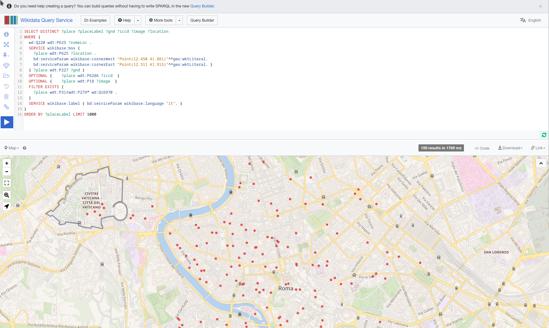
In this query:
-
We again ask for items at in the center of Rome (square bounding box cornerSW/NE).
-
We are only interested in items having an GND ID (
wdt:P227). -
We filtered for only items which are instance of (
wdt:P31) or subclass of (wdt:P279) of a religious building (wd:Q16970). This is non real equivalent for building=church in OSM, but close. -
We asked to list the Wikidata ID (
?place), its name (?placeLabel) in Italian, and its GND ID (?gnd).
nb. Obviously you can also look for more than one kind of building1.
We get back a nice list of 140 records. Ok, it‹s only 140 … not 270 ... but it's a start. Someone has to fix the other 130 ones where Wikidata has no GND information.
Here's a look at the output:
| place | placeLabel | gnd | iccd |
| wd:Q1631593 | Basilica di Sant'Andrea della Valle | 4458807-0 | |
| wd:Q1137391 | Basilica di Santa Maria in Trastevere | 4424041-7 | 15478 |
| wd:Q99309 | Pantheon | 4115786-2 | |
| wd:Q2031901 | Santa Maria in Vallicella | 4459147-0 | 15481 |
Save this data (menu Download Result / CSV file) as query.csv.
Now we have to combine the data we have from OpenStreetMap (the vectors) with the data from Wikidata (the IDs).
In order to make the join query, iand in order to have something visual, we use QGIS.
In QGIS, make a new Project and save it as ChurchesRome.qgz.
If you want to have a basic map layer, install the plugin QuickMapsServices (menu: Plugins / Install and Manage Plugins / All / Search: QuickMapServices / Install Plugin) and then add the OSM map (menu: Web / QuickMapsServices / OSM / OSM Standard).
If you want to display the latest archaeological findings, install it as WMS (menu: Layer / Add Layer / Add WMS/WMST Layer) and connect with the WMS source (menu: New):
| value | |
|---|---|
| name | Sepia & ArcheoSitar |
| url | https://api.mapbox.com/styles/v1/kewerner/cleh4lkpg003q01msrl463gd6/wmts?access_token=pk.eyJ1Ijoia2V3ZXJuZXIiLCJhIjoiY2lqMGprNjVmMDA0NnYwbTVibHh5bWx6aSJ9.zB8-7hnUeIeYJsqzOjJ2Fg |
If instead you want to display the Nolli map, install it as WMS, too:
| value | |
|---|---|
| name | Sepia & Nolli |
| url | https://api.mapbox.com/styles/v1/kewerner/clei8a8og000401mny1num8ol/wmts?access_token=pk.eyJ1Ijoia2V3ZXJuZXIiLCJhIjoiY2lqMGprNjVmMDA0NnYwbTVibHh5bWx6aSJ9.zB8-7hnUeIeYJsqzOjJ2Fg |
Click Ok, Connect, Add the »Sepia & ArcheoSitar« (or »Sepia & Nolli«) Layer and Close. You should see a nice background.
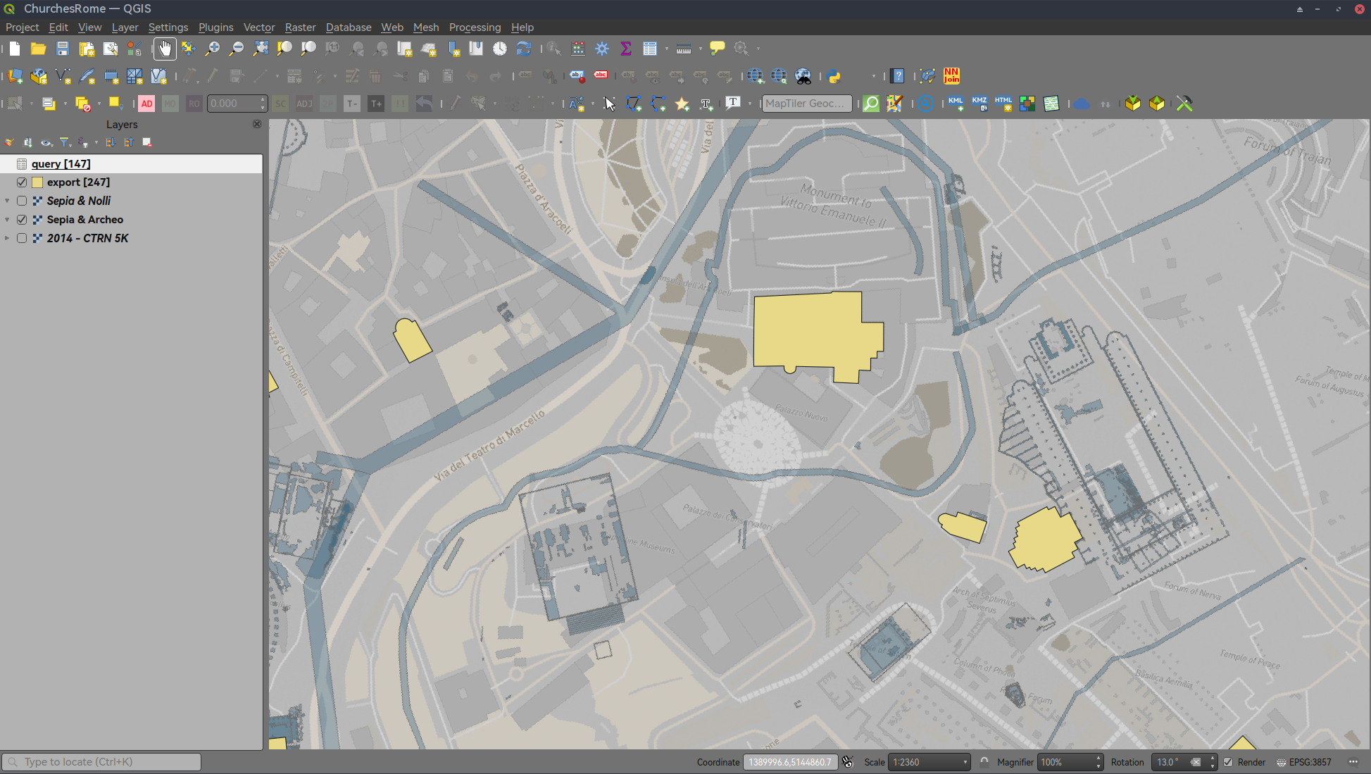
[ image ]
Now we import both tables as layers.
For the OSM data, import the export.geojson file: menu Add / Add Layer / Add Vector Layer and File / Source: export.geojson.
Leave the Options, as the default ones are just fine. Click Add and Close.
You now have a new layer called »export« on your map:
[ image ]
For the Wikidata data, import the the query.csv file: menu Add / Add Layer / Add Delimited Text Layer and File name: query.csv.
Leave File Format as CSV (comma separated values) but change Geometry Definition to "No geometry (attribute table only)".
Click Add and Close.
You now have a new layer called »query«.
We now have to mix the extended metadata information inside the Wikidata (our »query« layer) with the vector geometries from OSM. We will do this using a SQL query inside QGIS.
Choose Database / Database Manager and click on Virtual Layers / Project Layers. You now see our ›export‹ and ›query‹ layers we‹ve created.
Click on the ›export‹ layer and then menu SQL Window (2nd icon from top left).
The Query window opens.
Write the following query:
SELECT DISTINCT geometry, name, id, wikidata, query.image, query.*
FROM export
LEFT JOIN query on place='http://www.wikidata.org/entity/'||COALESCE(export.wikidata, '')
WHERE gnd NOT NULL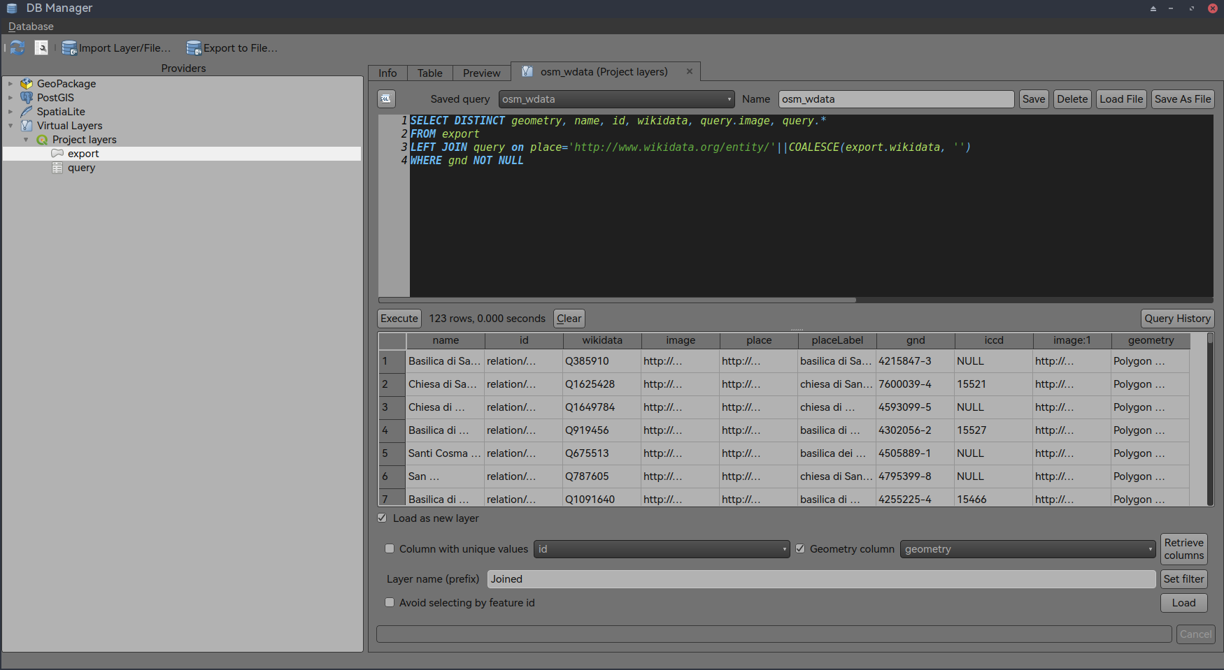
Choose Load as new layer and both Column with unique values: id and Geometry column: geometry.
Give Layer name as joined and click Load.
Close the DB Manager. The new layer ›Joined‹ will have 116 items:
[ image ]
Export the ›Joined‹ layer from QGIS as GeoJSON: hold the mouse over the layer and choose Export / Save vector layer as withthe ff. parameters:
| value | |
|---|---|
| Format | GeoJSON |
| Filename | joined.geojson |
| CRS | EPSG4326 - WGS 84 |
| Select fields to export | (all) |
| Persist layer metadata | (true) |
| Geometry type | automatic |
Leave Layer options in default and custom options blank, and Add saved file to map as false.
We now have the data and the vector piolygons together in one file.
We will need some webspace for hosting our GeoJSON and HTML files. Github works just fine. Otherwise contact your admin 👍
But we also need a map service like Leaflet, ArcGis or Mapbox which gives us the actual cartographic context. You wouldn't want to start your own server, would you?
Fortunately, there is ample choice of web map solutions. For this exercise, we use Mapbox, which is mostly free.
First, and obviously, create an account on mapbox.com.
Then, get a token for your project: https://account.mapbox.com/access-tokens/create and use it inside the following code for your index.html:
<!DOCTYPE html>
<html>
<head>
<meta charset="utf-8">
<title>Wikidata for Churches in Rome</title>
<meta content="initial-scale=1,maximum-scale=1,user-scalable=no" name="viewport">
<link href="https://api.mapbox.com/mapbox-gl-js/v2.13.0/mapbox-gl.css" rel="stylesheet">
<script src="https://api.mapbox.com/mapbox-gl-js/v2.13.0/mapbox-gl.js"></script>
<style>
body {
margin: 0;
padding: 0;
}
#map {
position: absolute;
top: 0;
bottom: 0;
width: 100%;
}
.mapboxgl-popup {
padding: 1em;
font: 12px/20px 'Helvetica Neue', Arial, Helvetica, sans-serif;
}
.mapboxgl-popup-content {
width: fit-content;
padding: 2em;
color: dimgray;
background-color: rgb(220, 220, 220);
border-radius: 8px;
border: thin outset white;
white-space: nowrap;
}
.mapboxgl-popup-content a {
color: dimgray;
text-decoration: none
}
span {
font-size: 110%;
}
img {
width: 200px;
border-radius: 5px;
border: thin inset white;
}
</style>
</head>
<body>
<div id="map"></div>
<script>
mapboxgl.accessToken = 'pk.YOUR_TOKEN_HERE'; //Put in YOUR actual token created in Mapbox!
// Create a new map.
const map = new mapboxgl.Map({
container: 'map',
// Choose from Mapbox's core styles, or make your own style with Mapbox Studio
style: 'mapbox://styles/kewerner/cleh4lkpg003q01msrl463gd6', //'mapbox://styles/mapbox/light-v10',
center: [12.481849, 41.897035],
zoom: 15,
hash: true
});
map.on('load', () => {
// Add a source for the state polygons.
map.addSource('churches', {
'type': 'geojson',
'data': 'joined.geojson'
});
// Add a layer showing the state polygons.
map.addLayer({
'id': 'churches-layer',
'type': 'fill',
'source': 'churches',
'paint': {
'fill-color': 'rgba(250,200,100,0.5)',
'fill-outline-color': 'white'
}
});
// When a click event occurs on a feature in the states layer,
// open a popup at the location of the click, with description
// HTML from the click event's properties.
map.on('click', 'churches-layer', (e) => {
new mapboxgl.Popup()
.setLngLat(e.lngLat)
.setHTML(
'<b><span>' + e.features[0].properties.name + '</span></b>' +
'<br/>' +
'<br/><b>GND ' + e.features[0].properties.gnd + '</b>' +
'<br/>⯈ <a href="https://aleph.mpg.de/F?func=find-a&find_code=PER&request=&request_op=AND&find_code=IGD&request=' + e.features[0].properties.gnd + '&request_op=AND&find_code=WKO&request=&request_op=AND&find_code=WSW&request=&filter_code_1=WSP&filter_request_1=&filter_code_2=WYR&filter_request_2=&filter_code_3=WYR&filter_request_3=&filter_code_4=WEF&filter_request_4=&local_base=KUB01&filter_code_7=WEM&filter_code_8=WAK">Library</a>' +
'<br/>⯈ <a href="https://dlib.biblhertz.it/show.html?gnd=https://gn.biblhertz.it/fotothek/api/normdatei/architectur/' + e.features[0].properties.gnd + '">Photo Collection</a>' +
'<br/>' +
'<br/><b>WData ' + e.features[0].properties.wikidata + '</b>' +
'<br/>⯈ <a href="' + e.features[0].properties.place + '">Wikidata</a>' +
'<br/>' +
'<br><img src="' + e.features[0].properties.image + '"/>'
)
.addTo(map);
});
// Change the cursor to a pointer when
// the mouse is over the states layer.
map.on('mouseenter', 'states-layer', () => {
map.getCanvas().style.cursor = 'pointer';
});
// Change the cursor back to a pointer
// when it leaves the states layer.
map.on('mouseleave', 'states-layer', () => {
map.getCanvas().style.cursor = '';
});
});
// Add geolocate control to the map.
map.addControl(
new mapboxgl.GeolocateControl({
positionOptions: {
enableHighAccuracy: true
},
// When active the map will receive updates to the device's location as it changes.
trackUserLocation: true,
// Draw an arrow next to the location dot to indicate which direction the device is heading.
showUserHeading: true
})
);
</script>
</body>
</html>Upload both index.html and joined.geojson and you're done.
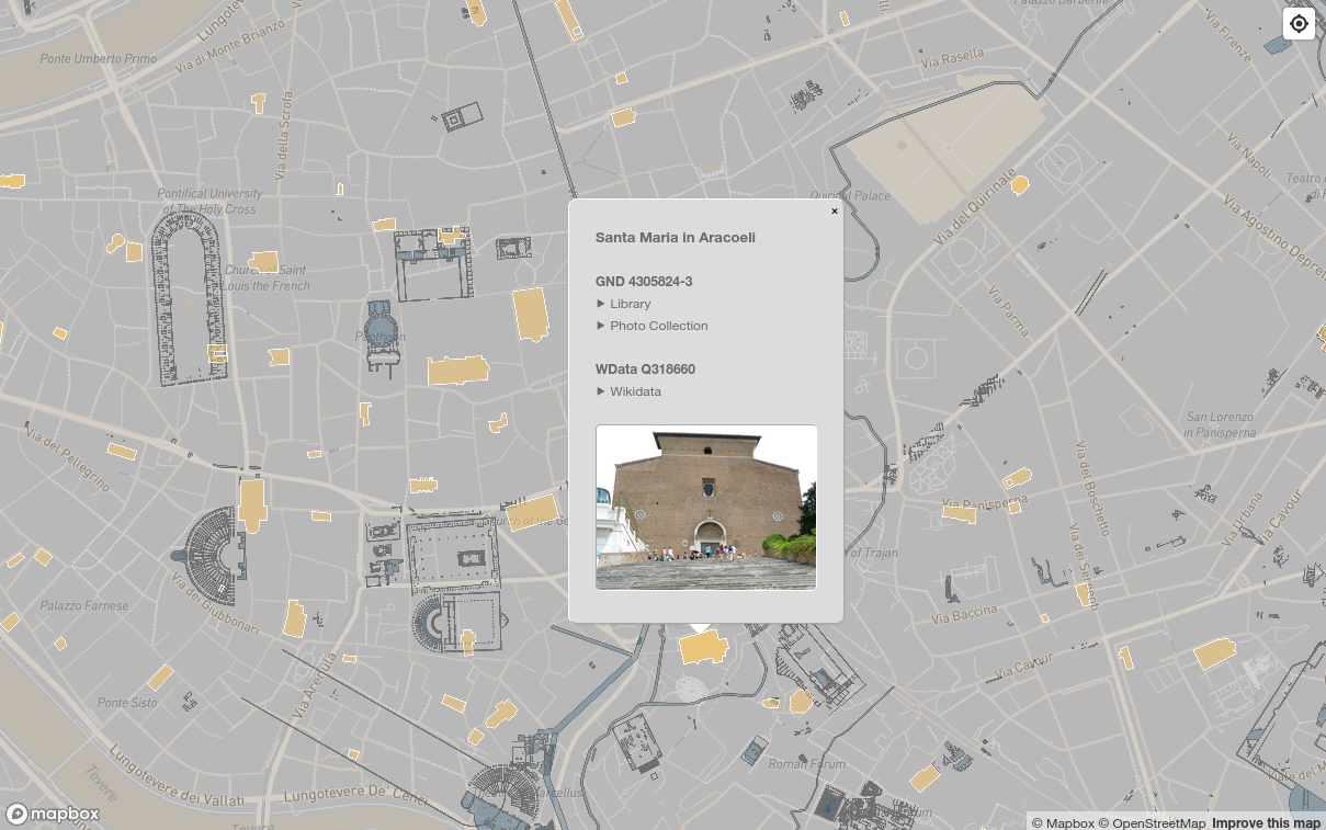
A web version here: http://maps.kewerner.name/datathink/
You have now:
- a web map with your selected polygons
- links to data for these resources in the photographic collection and the library
- a link to WikiData for any other relevant resource
Keep in mind that this is only a visualization, and a rather crude one: you still manually have to click the links.
But the trick of connecting data from different information systems with a map presentation by using a wikidata ID can be useful in many scenarios.
--kew 24/ii ab n.d. mmxxiii
Footnotes
-
The relevant line instead of
?place wdt:P31/wdt:P279* wd:Q16970 .would then be:VALUES ?instance { wd:Q24398318 wd:Q14752696 wd:Q109607 wd:Q16560 wd:Q16970 wd:Q160742 wd:Q23413 wd:Q1128397 wd:Q1195705 wd:Q12518 wd:Q839954 wd:Q815448 wd:Q120560 wd:Q1649060 wd:Q580499 wd:Q19899465 wd:Q483453 wd:Q557141 wd:Q44613 wd:Q82117 }. ↩