1) Image Segmentation
Image segmentation groups similar pixels into segments. The segmentation delivers closed contours capturing the outlines of visible objects (Figure 1). In this wiki, the use of Multiscale Combinatorial Grouping (MCG) is described. MCG is an open source method developed by Berkley University, which we have modified for georeferenced remote sensing imagery. The source code is pre-complied to be used in Matlab under Linux.

Figure 1: Image segmentation delivers closed contours (right) capturing the outlines of visible objects in a remote sensing image (left).
After applying MGC image segmentation, we convert the MCG raster to vector lines (Figure 2) and apply line filtering (Figure 3). These steps can be conducted in any GIS such as the free and open source QGIS or the commercial ESRI ArcGIS.

Figure 2: Remote sensing image (left). MCG image segmentation result in raster format (middle). MCG lines derived from raster to vector conversion (right).

Figure 3: MCG line filtering reducing the line count by 80%.
- RGB orthoimage raster
.tif -
World file
.tfw
- image segmentation lines without attributes
.shp
- Install Matlab & MCG image segmentation
- Prepare input orthoimage
- Run MCG
- Raster to vector conversion
- Line filtering (optional)
-
Install Matlab
- Instructions on how to install the software are provided on the Matlab website
-
Download our modified MCG version from GitHub to your Linux computer and save in a
MCGfolder
Depending on the memory capacity of your computer, you might have to clip your RGB orthoimage raster (.tif) into tiles that do not exceed 10,000 x 10,000 pixels. The tiles must be quadratic.
-
Clip orthoimage into quadratic tiles of max. 10,000 x 10,000 pixels
-
Open your orthoimage in QGIS
-
Right click your orthoimage |
Export|Save As...| EnableCreate VRT| Define a file name with...| Set VRT Tilesmax columnsandmax rowsto10000or lower | ClickOK
- Alternatively, you can clip your orthoimage in the
OSGeo4Wshell withgdalwarp -crop_to_cutline -cutline clip.shp orthoimage.tif orthoimage_clipped.tif
- Alternatively, you can clip your orthoimage in the
-
-
Create a world file for each tiled orthoimage
- Open
OSGeo4Wshell- Select the Windows start button > type
OSGeo4W - Change the shells's working directory to your tiled orthoimages
-
cd path_to_folder
-
- Create a
.tfwfile describing the georeference of your orthoimage. The orthoimage will not be changed.-
gdal_translate -co "TFW=YES" orthoimage.tif orthoimage_translated.tif
-
- Select the Windows start button > type
- Open
-
Save your RGB orthoimage raster (
.tif) and the corresponding world file (.tfw) both having the same name to\MCG\pre-trained\demos\data -
Open Matlab
-
Add the path of the downloaded MCG folder in Matlab
- Right click on the MCG folder |
Add to Path|Selected Folders and Subfolders
- Right click on the MCG folder |
-
Change the EPSG code in
\MCG\pre-trained\scripts\geotiffwrapper.mto that of your orthoimage-
A.ProjectedCSTypeGeoKey= your EPSG code
-
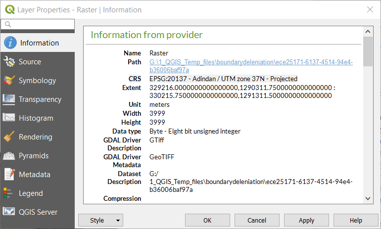
You can check the EPSG code of your orthoimage by opening it in QGIS and reading the EPSG code from the bottom right corner

or by right clicking your orthoimage |
Properties|Information
-
-
Set all parameters under
%%Predefine variables%%in\MCG\pre-trained\demos\mcg.m-
k: value between 0 and 1 that regulates over- and under-segmentations.- Low values produce more boundaries and thus more over-segmentation. For our test data of 0.25 m GSD, we set
k = 0.1to produce over-segmentation. This setting creates outlines around the majority of visible objects. Tests with higher values (k = 0.3andk = 0.5) resulting in less over-segmentation show that visible object outlines are partly missed, while irrelevant lines around small objects are still produced. For high-resolution imagery of 0.05 cm GSD, we setk = 0.3ork = 0.4.
- Low values produce more boundaries and thus more over-segmentation. For our test data of 0.25 m GSD, we set
-
ext: appendix added to output boundary map files. You can chose any text to later identify your results. -
myDir: path to input data directory -
outDir: path to store output data
-
-
Run
\MCG\pre-trained\demos\mcg.m- Right click on
mcg.m|run
- MCG will be applied to each orthoimage stored in
myDir
- Right click on
-
Merge MCG raster tiles (optional)
- Note: only required in case you tiled your orthoimage before applying MCG
- Open Search (Ctrl + F) and search for
Mosaic To New Raster - Set the MCG raster tiles as
Input Rasters| Define anOutput Location| DefineRaster Dataset Name with Extension| SetNumber of Bandsto 1
The result of mcg.m are binary rasters, in which the value 1 is assigned to boundary pixels and 0 to not boundary pixels. These rasters need to converted to a vector line format ([Figure 2](Figure 2)) and ([Figure 4](Figure 4)).

Figure 4: Raster to vector conversion, which converts the binary MCG boundary map (black and white pixels) to a vector line layer (red lines).
Convert raster to vector
-
Open ArcGIS
-
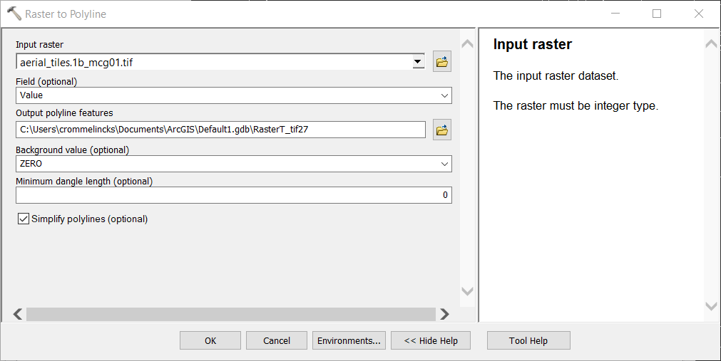
Open Search (Ctrl + F) and search for
Raster to Polyline
-
Run
Raster to Polylineon the MCG raster, changing only theInput rastervariable
To reduce the number of irrelevant lines produced through over-segmentation, lines can be simplified through filtering: lines around areas smaller than 30 m2 are merged to the neighboring segments, which reduces the line count by roughly 80%. According to our visual inspections, this post-processing removes artefacts in the segmentation results and keeps outlines of large objects being more relevant for cadastral mapping.
Simplify segment lines
- Download the ArcGIS toolbox from Github that contains our tool
SimplifySegmentation-
SimplifySegmentationis a tool created with theModel Builderthat combines different ArcGIS toolbox functionalities:
-
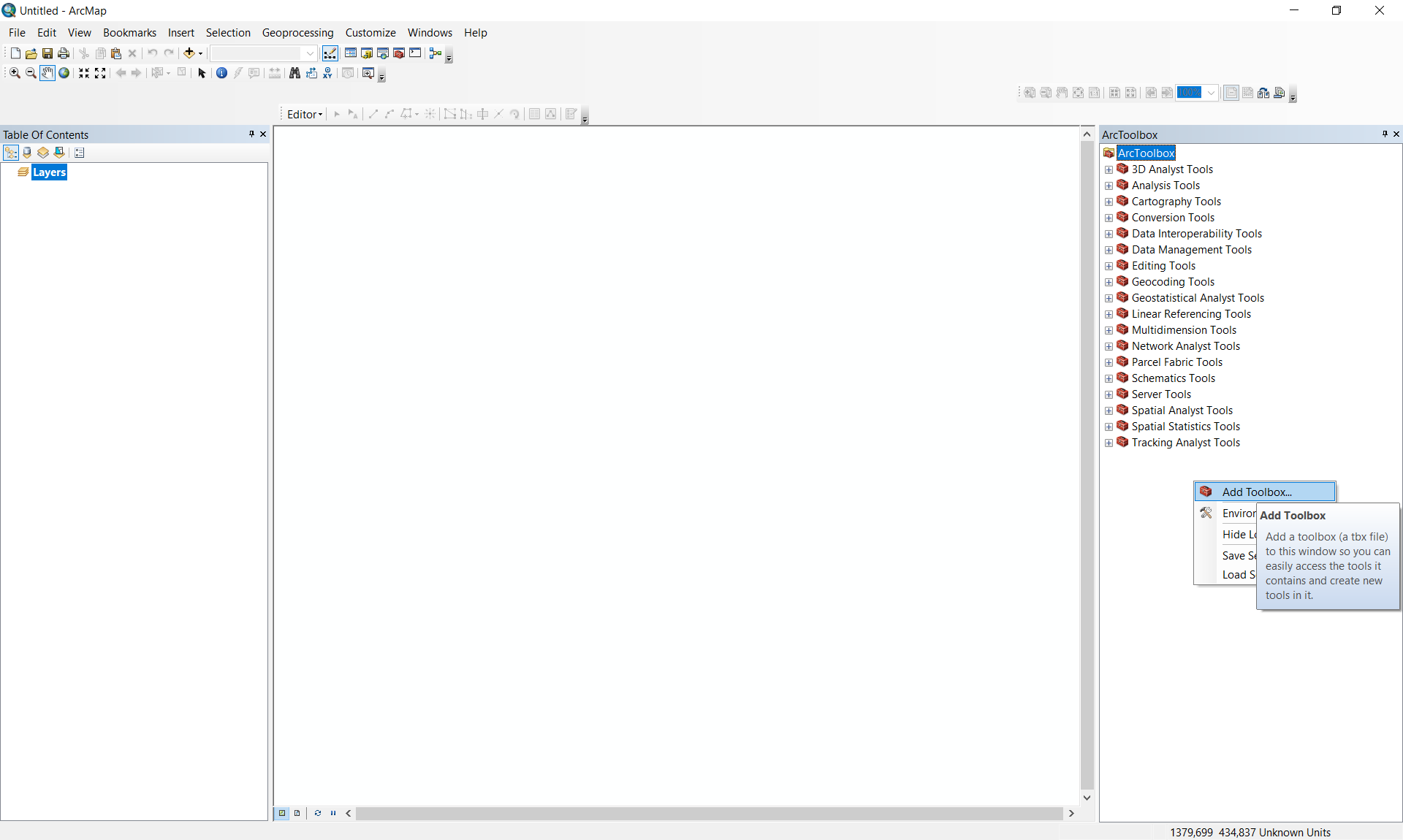
- Add the downloaded toolbox in ArcGIS
- right click in
ArcToolboxwindow |Add Toolbox...
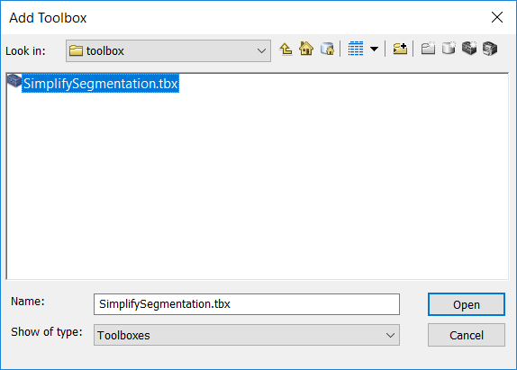
- Load the downloaded toolbox

- right click in
- Open the tool
SimplifySegmentation, which should now appear as a new toolbox in yourArcToolbox
- Run
SimplifySegmentation-
Select lines to be simplified as
Input Lines -
Set path to store simplified lines as
Output Lines

-
The steps described in ArcGIS can also be performed in free GIS software such as QGIS or the OSGeo4W.
Merge rasters
- Download the Python gdal_merge script to your gdal libraries directory
- Replace the following parameters
output.tif,tile1.tif,tile2.tifwith your file names and run the following in the OSGeo4W Shell
import subprocess
merge_command = ["python", "gdal_merge.py", "-o", "output.tif", "tile1.tif", "tile2.tif", "tile3.tif"]
subprocess.call(merge_command)
- Refer to the GDAL documentation for further details
Convert raster to vector
- Refer to instructions on Stack Exchange, in which we propose to apply the following steps:
- Replace all no data values
processing.runalg('grass:r.mapcalculator', {"amap": gPb_rlayer, "formula": "if(A>0, 1, null())", "GRASS_REGION_PARAMETER": "%f,%f,%f,%f" % (xmin, xmax, ymin, ymax), "GRASS_REGION_CELLSIZE_PARAMETER": 1, "outfile": mapcalc})- Thin raster layer to thin non-null cells
processing.runalg('grass7:r.thin', {"input": mapcalc, "GRASS_REGION_PARAMETER": "%f,%f,%f,%f" % (xmin, xmax, ymin, ymax), "output": thinned})- Raster to vector conversion
processing.runalg('grass7:r.to.vect',
                {"input": thinned,
                 "type": 0,
                 "GRASS_OUTPUT_TYPE_PARAMETER": 2,
                 "GRASS_REGION_PARAMETER": "%f,%f,%f,%f" % (xmin, xmax, ymin, ymax),
                 "output": centerlines})
Simplify segment lines
- We created the same
SimplifySegmentationtool with theProcessing Modelerin QGIS that we created before in ArcGIS. Download the QGIS toolbox from Github. However, we observed that it runs less stable for larger data sets.
- In comparison to the , we have modified the following scripts:
-
\MCG\pre-trained\demos\mcg.m-> to call MCG image segmentation -
\MCG\pre-trained\scripts\geotiffwrapper.m-> to define EPSG code in input raster data -
\MCG\pre-trained\scripts\geotiffwrite.m-> to write EPSG code from input to output raster
-
- The original MGC source code developed by Berkley University that we have modified for georeferenced remote sensing imagery is publically available under the GNU General Public License
